# A tibble: 122 × 4
   last_name  party num_votes agree
   <chr>      <chr>     <dbl> <dbl>
 1 Alexander  R           118 0.890
 2 Blunt      R           128 0.906
 3 Brown      D           128 0.258
 4 Burr       R           121 0.893
 5 Baldwin    D           128 0.227
 6 Boozman    R           129 0.915
 7 Blackburn  R           131 0.885
 8 Barrasso   R           129 0.891
 9 Bennet     D           121 0.273
10 Blumenthal D           128 0.203
# ℹ 112 more rows
Exercise
Add a new column to the data frame, called diff_agree, which subtracts agree and agree_pred. How would you create abs_diff_agree, defined as the absolute value of diff_agree? Your code:
Filter the data frame to only get senators for which we have information on fewer than (or equal to) five votes. Your code:
Filter the data frame to only get Democrats who agreed with Trump in at least 30% of votes. Your code:
Add a new column to the data frame, called diff_agree, which subtracts agree and agree_pred. How would you create abs_diff_agree, defined as the absolute value of diff_agree? Your code:
trump_scores |>mutate(diff_agree = agree - agree_pred) |>select(last_name, matches("agree")) # just for clarity
Filter the data frame to only get senators for which we have information on fewer than (or equal to) five votes. Your code:
trump_scores |>filter(num_votes <=5)
# A tibble: 5 × 8
  bioguide last_name    state party num_votes agree agree_pred margin_trump
  <chr>    <chr>        <chr> <chr>     <dbl> <dbl>      <dbl>        <dbl>
1 H000273  Hickenlooper CO    D             2   0       0.0302        -4.91
2 H000601  Hagerty      TN    R             2   0       0.115         26.0
3 K000377  Kelly        AZ    D             5   0.2     0.262          3.55
4 L000571  Lummis       WY    R             2   0.5     0.225         46.3
5 T000278  Tuberville   AL    R             2   1       0.123         27.7
Filter the data frame to only get Democrats who agreed with Trump in at least 30% of votes. Your code:
trump_scores |>filter(party =="D"& agree >=0.3)
# A tibble: 11 × 8
   bioguide last_name state party num_votes agree agree_pred margin_trump
   <chr>    <chr>     <chr> <chr>     <dbl> <dbl>      <dbl>        <dbl>
 1 D000607  Donnelly  IN    D            83 0.542      0.833        19.2
 2 H001069  Heitkamp  ND    D            84 0.548      0.915        35.7
 3 J000300  Jones     AL    D            68 0.353      0.845        27.7
 4 K000383  King      ME    D           129 0.372      0.441        -2.96
 5 M001170  McCaskill MO    D            83 0.458      0.830        18.6
 6 M001183  Manchin   WV    D           129 0.504      0.893        42.2
 7 N000032  Nelson    FL    D            83 0.434      0.568         1.20
 8 R000608  Rosen     NV    D           136 0.346      0.604        -2.42
 9 S001191  Sinema    AZ    D           135 0.504      0.398         3.55
10 T000464  Tester    MT    D           129 0.302      0.805        20.4
11 W000805  Warner    VA    D           129 0.349      0.401        -5.32
Exercise
Arrange the data by diff_pred, the difference between agreement and predicted agreement with Trump. (You should have code on how to create this variable from the last exercise). Your code:
# A tibble: 2 × 2
  party max_abs_diff
  <chr>        <dbl>
1 R            0.877
2 D            0.503
Exercise
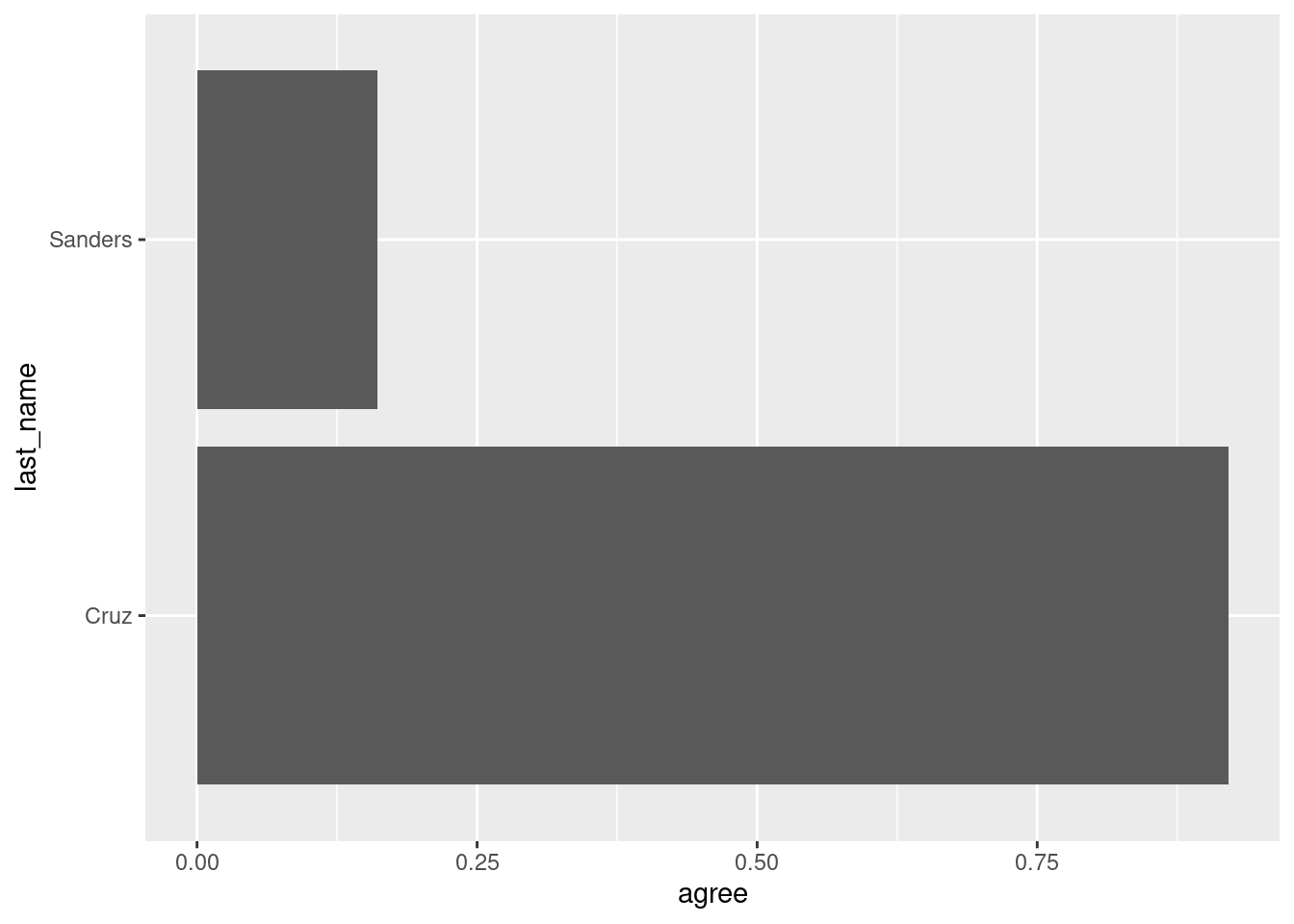
Draw a column plot with the agreement with Trump of Bernie Sanders and Ted Cruz. What happens if you use last_name as the y aesthetic mapping and agree in the x aesthetic mapping? Your code:
Code
# setup: this step was executed before the exercisetrump_scores_ss <- trump_scores |>filter(num_votes >=10)
ggplot(trump_scores_ss |>filter(last_name %in%c("Cruz", "Sanders")),aes(y = last_name, x = agree)) +geom_col()
Calculate \(2\times A\) and \(-3 \times B\). Again, do one by hand and the other one using R. \[A= \begin{bmatrix}
1 & 4 & 8 \\
0 & -1 & 3
\end{bmatrix}\]\[ B = \begin{bmatrix}
-15 & 1 & 5 \\
2 & -42 & 0 \\
7 & 1 & 6
\end{bmatrix}\]
# A tibble: 4 × 2
  region           med_corr
  <chr>               <dbl>
1 Caribbean          0.301
2 South America      0.531
3 Central America    0.734
4 Northern America   0.0505
Exercise
Convert back gdp_long to a wide format using pivot_wider(). Check out the help file using ?pivot_wider. Your code:
Code
# setup: these steps were executed before the exerciselibrary(readxl)gdp <-read_excel("data/wdi_gdp_ppp.xlsx")gdp_long <- gdp |>pivot_longer(cols =-c(country_name, country_code), names_to ="year", values_to ="wdi_gdp_ppp", names_transform = as.integer)
gdp_long |>pivot_wider(id_cols =c(country_name, country_code), # can omit in this case toovalues_from = wdi_gdp_ppp, names_from = year)
# A tibble: 266 × 35
   country_name        country_code   `1990`   `1991`   `1992`   `1993`   `1994`
   <chr>               <chr>           <dbl>    <dbl>    <dbl>    <dbl>    <dbl>
 1 Aruba               ABW           2.03e 9  2.19e 9  2.32e 9  2.48e 9  2.69e 9
 2 Africa Eastern and… AFE           9.41e11  9.42e11  9.23e11  9.19e11  9.35e11
 3 Afghanistan         AFG          NA       NA       NA       NA       NA
 4 Africa Western and… AFW           5.76e11  5.84e11  5.98e11  5.92e11  5.91e11
 5 Angola              AGO           6.85e10  6.92e10  6.52e10  4.95e10  5.02e10
 6 Albania             ALB           1.59e10  1.14e10  1.06e10  1.16e10  1.26e10
 7 Andorra             AND          NA       NA       NA       NA       NA
 8 Arab World          ARB           2.19e12  2.25e12  2.35e12  2.41e12  2.48e12
 9 United Arab Emirat… ARE           2.01e11  2.03e11  2.10e11  2.12e11  2.27e11
10 Argentina           ARG           4.61e11  5.04e11  5.43e11  5.88e11  6.22e11
# ℹ 256 more rows
# ℹ 28 more variables: `1995` <dbl>, `1996` <dbl>, `1997` <dbl>, `1998` <dbl>,
#   `1999` <dbl>, `2000` <dbl>, `2001` <dbl>, `2002` <dbl>, `2003` <dbl>,
#   `2004` <dbl>, `2005` <dbl>, `2006` <dbl>, `2007` <dbl>, `2008` <dbl>,
#   `2009` <dbl>, `2010` <dbl>, `2011` <dbl>, `2012` <dbl>, `2013` <dbl>,
#   `2014` <dbl>, `2015` <dbl>, `2016` <dbl>, `2017` <dbl>, `2018` <dbl>,
#   `2019` <dbl>, `2020` <dbl>, `2021` <dbl>, `2022` <dbl>
Exercise
There is a dataset on country’s CO2 emissions, again from the World Bank (2023), in “data/wdi_co2.csv”. Load the dataset into R and add a new variable with its information, wdi_co2, to our qog_plus data frame. Finally, compute the average values of CO2 emissions per capita, by country. Tip: this exercise requires you to do many steps—plan ahead before you start coding! Your code:
Code
# setup: these steps were executed before the exerciselibrary(tidyverse)qog <-read_csv("data/sample_qog_bas_ts_jan23.csv")gdp <- readxl::read_excel("data/wdi_gdp_ppp.xlsx")gdp_long <- gdp |>pivot_longer(cols =-c(country_name, country_code),names_to ="year",values_to ="wdi_gdp_ppp", names_transform = as.integer)qog_plus <-left_join(qog, gdp_long,by =c("ccodealp"="country_code","year"))
Load data (notice the .csv format):
emissions <-read_csv("data/wdi_co2.csv")
Rows: 266 Columns: 35
── Column specification ────────────────────────────────────────────────────────
Delimiter: ","
chr  (2): country_name, country_code
dbl (31): 1990, 1991, 1992, 1993, 1994, 1995, 1996, 1997, 1998, 1999, 2000, ...
lgl  (2): 2021, 2022

ℹ Use `spec()` to retrieve the full column specification for this data.
ℹ Specify the column types or set `show_col_types = FALSE` to quiet this message.
Pivot data to long, creating the “wdi_co2” variable:
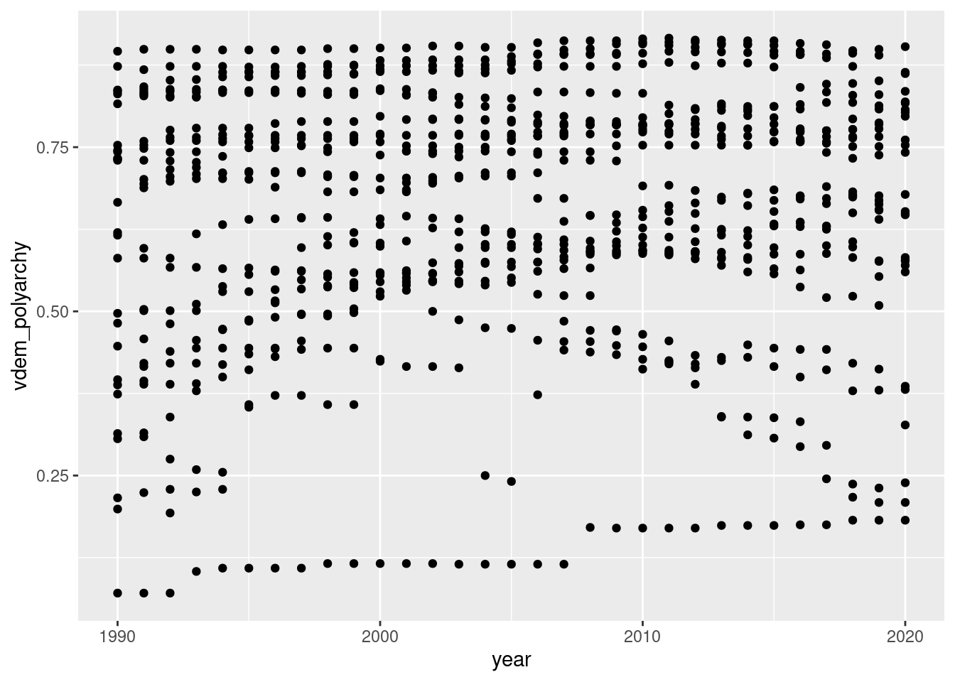
Warning: Removed 248 rows containing missing values or values outside the scale range
(`geom_point()`).
Exercise
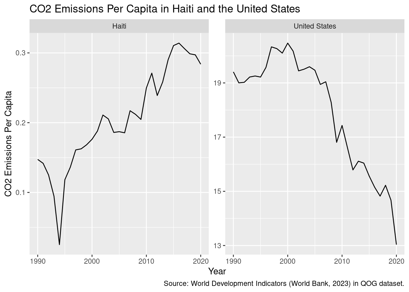
Using your merged dataset from the previous section, plot the trajectories of C02 per capita emissions for the US and Haiti. Use adequate scales.
ggplot(qog_plus2 |>filter(cname %in%c("Haiti", "United States")), aes(x = year, y =1000* wdi_co2 / wdi_pop)) +geom_line() +facet_wrap(~cname, scales ="free_y") +labs(x ="Year", y ="CO2 Emissions Per Capita",title ="CO2 Emissions Per Capita in Haiti and the United States",caption ="Source: World Development Indicators (World Bank, 2023) in QOG dataset.")
5. Functions
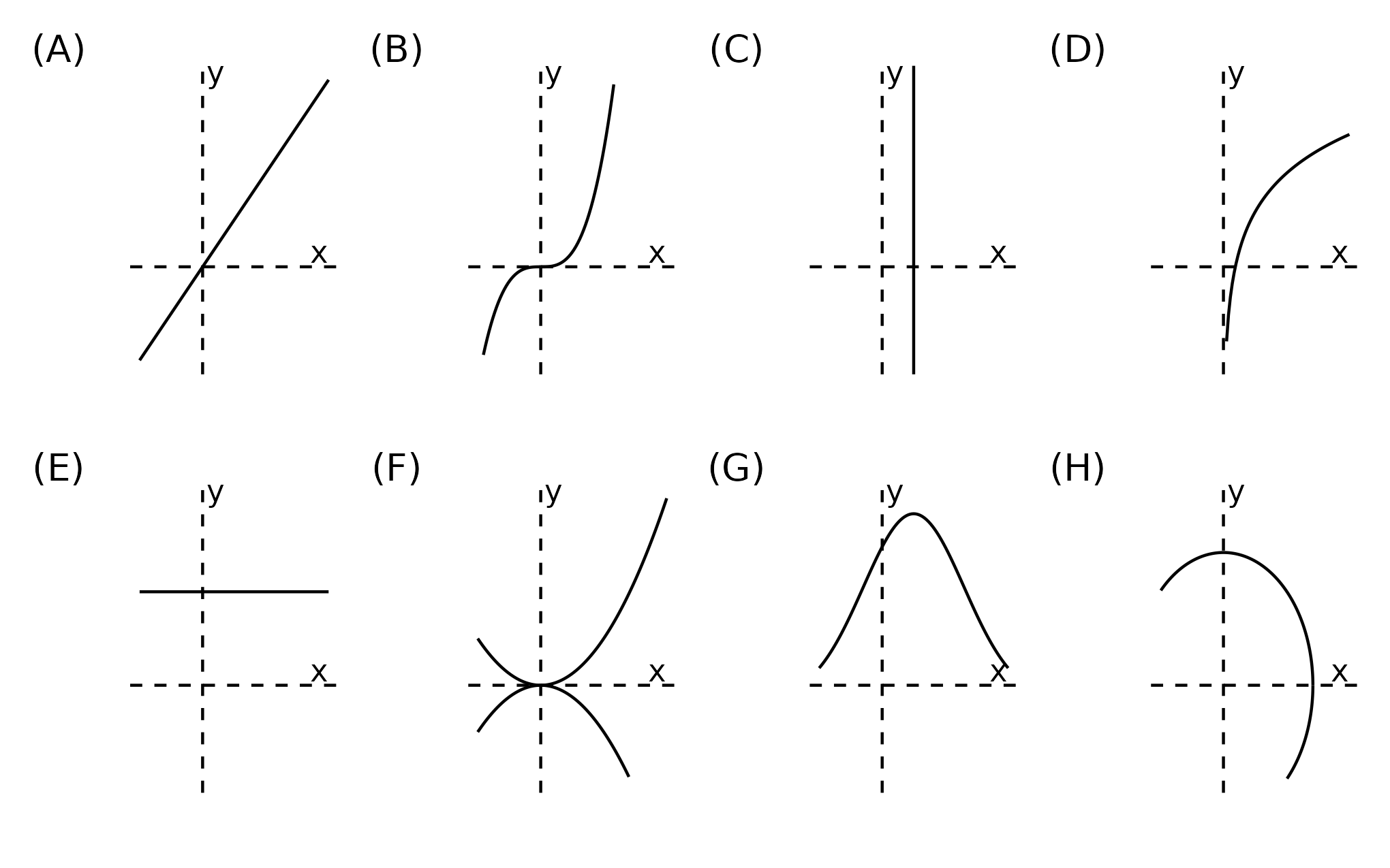
Exercise When graphed, vertical lines cannot touch functions at more than one point. Why? Which of the following represent functions?
Figure 1: Vertical line test: examples.
Function ✅
Function ✅
NOT a function 🚫
Function ✅
Function ✅
NOT a function 🚫
Function ✅
NOT a function 🚫
Exercise
Create a function that calculates the area of a circle from its diameter. So your_function(d = 6) should yield the same result as the example above. Your code:
Code
# setup: these steps were executed before the exercisecirc_area_r <-function(r){ pi * r ^2}circ_area_r(r =3)
[1] 28.27433
circ_area_d <-function(d){ pi * (d/2) ^2}circ_area_d(d =6)
[1] 28.27433
Exercise
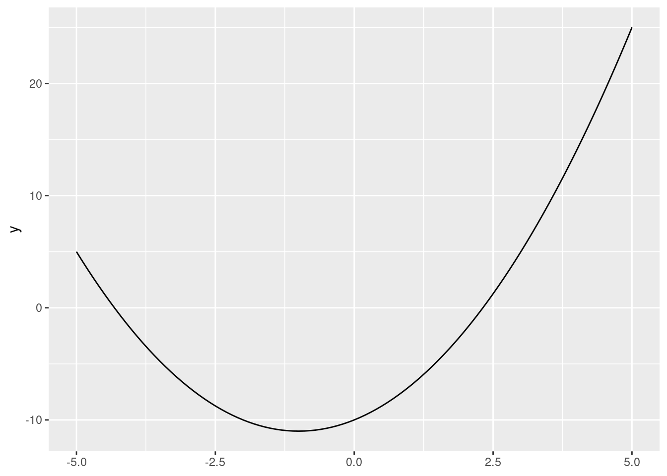
Graph the function \(y = x^2 + 2x - 10\), i.e., a quadratic function with \(a=1\), \(b=2\), and \(c=-10\). Next, try switching up these values and the xlim = argument. How do they each alter the function (and plot)?
Code
# setup: these steps were executed before the exerciselibrary(ggplot2)
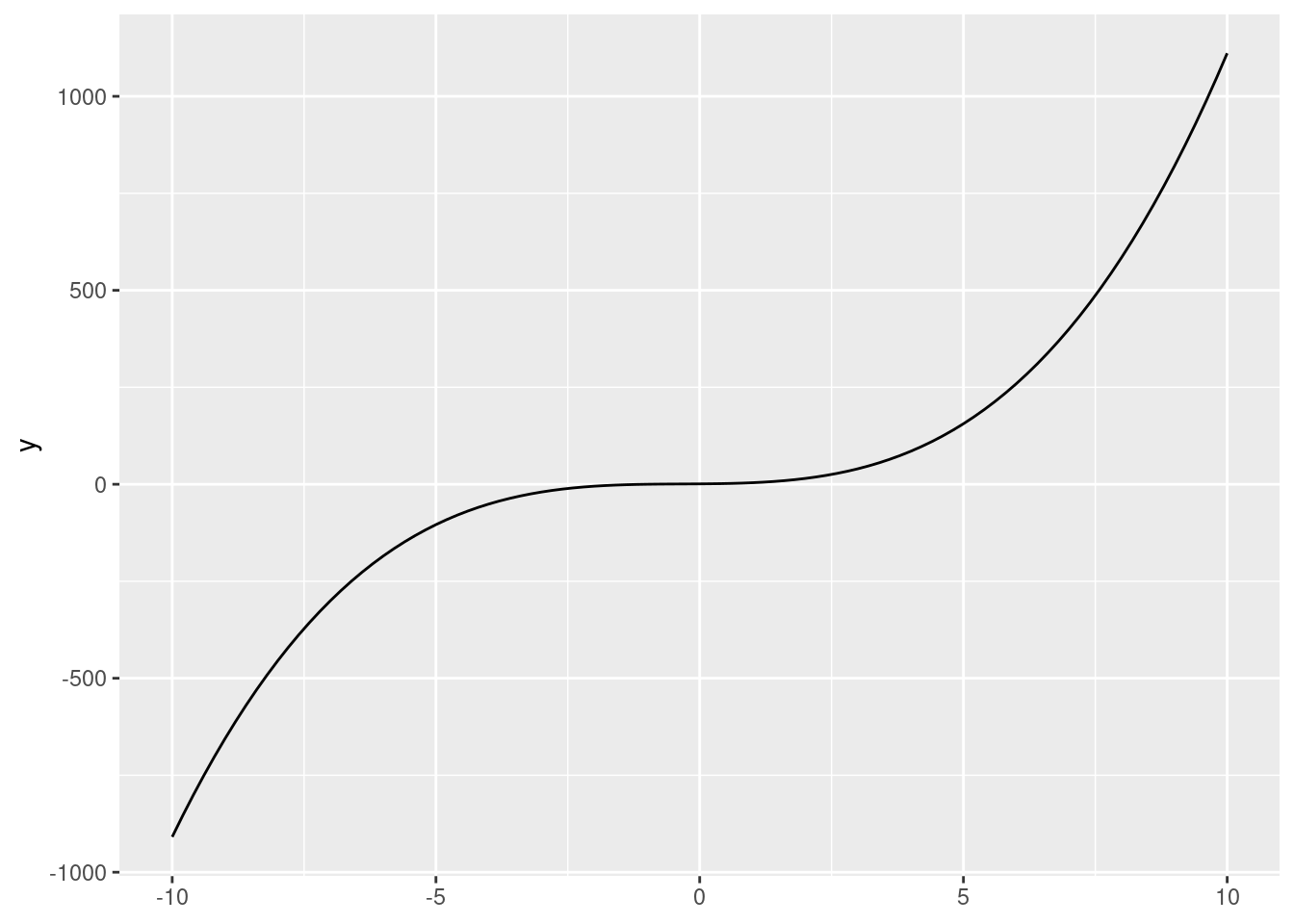
We’ll briefly introduce Desmos, an online graphing calculator. Use Desmos to graph the following function \(y = 1x^3 + 1x^2 + 1x + 1\). What happens when you change the \(a\), \(b\), \(c\), and \(d\) parameters?
(we’ll show how to do this in R here, but you could use Desmos)
Graph \(y = 1x^3 + 1x^2 + 1x + 1\).
ggplot() +stat_function(fun =function(x){x^3+ x^2+ x +1},xlim =c(-10, 10))
Solve the problems below, simplifying as much as you can. \[log_{10}(1000)\]\[log_2(\dfrac{8}{32})\]\[10^{log_{10}(300)}\]\[ln(1)\]\[ln(e^2)\]\[ln(5e)\]
log10(1000)
[1] 3
log2(8/32)
[1] -2
10^(log10(300))
[1] 300
log(1)
[1] 0
log(exp(2))
[1] 2
log(5*exp(1))
[1] 2.609438
Exercise
Compute g(f(5)) using the definitions above. First do it manually, and then check your answer with R.
Code
# setup: these steps were executed before the exercisef <-function(x){x ^2}g <-function(x){x -3}
\[f(5) = 5^2 = 25\]\[g(25) = 25 - 3 = 22\]
g(f(5)) # no pipeline approach
[1] 22
f(5) |>g() # pipeline approach
[1] 22
6. Calculus
Exercise
Use the slope formula to calculate the rate of change between 5 and 6.
Use the slope formula to calculate the rate of change between 5 and 5.5.
Use the slope formula to calculate the rate of change between 5 and 5.1.
(6^2-5^2) / (6-5)
[1] 11
(5.5^2-5^2) / (5.5-5)
[1] 10.5
(5.1^2-5^2) / (5.1-5)
[1] 10.1
Exercise
Use the differentiation rules we have covered so far to calculate the derivatives of \(y\) with respect to \(x\) of the following functions:
\(y = 2x^2 + 10\)
\(y = 5x^4 - \frac{2}{3}x^3\)
\(y = 9 \sqrt x\)
\(y = \frac{4}{x^2}\)
\(y = ax^3 + b\), where \(a\) and \(b\) are constants.
\(y = \frac{2w}{5}\)
\(4x\) (sum rule, constant rule, coefficient rule, power rule)
\(20x^3-2x^2\) (sum rule, coefficient rule, power rule)
\(\frac{-9}{2\sqrt x}\) (power rule)
\(-\frac{8}{x^3}\) (coefficient rule, power rule)
\(3ax^2\) (sum rule, constant rule, coefficient rule, power rule)
So we conclude that, for the \([-6, 6]\) interval, the global minimum is at the lower bound (\(x=-6\)) and the global maximum is at the critical point at \(x=-2\).
Evaluate the CDF of \(Y \sim U(-2, 2)\) at point \(y = 1\). Use the formula and punif().
\[A = F(1) = P(Y\leq 1) = 3 \cdot(1/4) = 0.75\]
punif(q =1, min =-2, max =2)
[1] 0.75
Exercise
What is the probability of obtaining a value above 1.96 or below -1.96 in a standard normal probability distribution? Hint: use the pnorm() function.
pnorm(-1.96) + (1-pnorm(1.96))
[1] 0.04999579
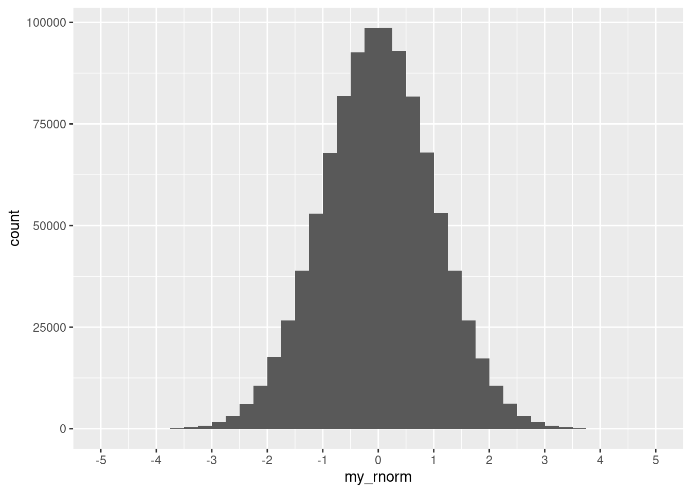
Exercise
Compute and plot my_rnorm, a vector with one million draws from a Normal distribution \(Z\) with mean equal to zero and standard deviation equal to one (\(Z\sim N(0,1)\)). You can recycle code from what we did for the uniform distribution!
What score (out of 10) would you give Barbie or Oppenheimer? Write your score in one sentence (e.g., I would give Barbie seven of ten stars.) If you have not seen either, write a sentence about which you would like to see more.
Store that text as a string (string3) and combine it with our existing cat_string to produce a new concatenated string called cat_string2. Finally, count the total number of characters within cat_string2. Your code:
Code
# setup: these steps were executed before the exerciselibrary(stringr)my_string <-"I know people who have seen the Barbie movie 2, 3, even 4 times!"my_string2 <-"I wonder if they have seen Oppenheimer, too."cat_string <-str_c(my_string, my_string2, sep =" ")
string3 <-"I would give Barbie 7 out of 10 stars."string3
[1] "I know people who have seen the Barbie movie 2, 3, even 4 times! I wonder if they have seen Oppenheimer, too. I would give Barbie 7 out of 10 stars."
str_length(cat_string2)
[1] 148
Exercise
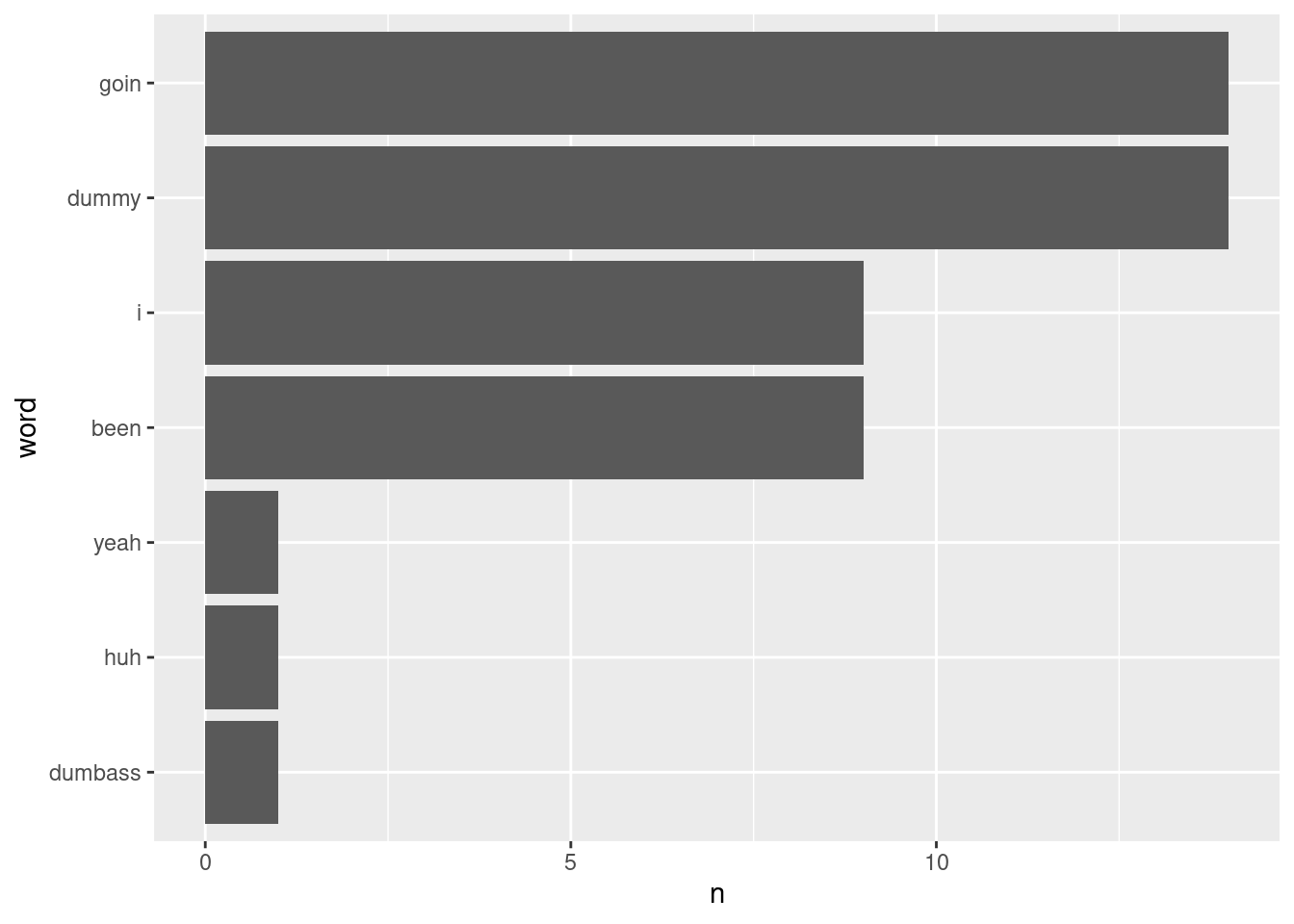
Look up the lyrics to your favorite song at the moment (no guilty pleasures here!). Then, follow the process described above to count the words: store the text as a string, convert to a tibble, tokenize, and count.
When you are done counting, create a visualization for the chorus using the ggplot code above. Your code:
Store the text as a string.
library(tidytext)dummy <-c("I been goin' dummy (Huh)","I been goin' dummy (Goin' dummy)","I been goin' dummy (Goin' dummy)","I been goin' dummy (Goin' dummy)","I been goin' dummy (Yeah)","I been goin' dummy (Goin' dummy)","I been goin' dummy (Goin' dummy)","I been goin' dummy","Dumbass, I been goin' dummy")
Convert to a tibble.
dummy_df <-tibble(line =1:9, text = dummy)dummy_df
# A tibble: 9 × 2
   line text
  <int> <chr>
1     1 I been goin' dummy (Huh)
2     2 I been goin' dummy (Goin' dummy)
3     3 I been goin' dummy (Goin' dummy)
4     4 I been goin' dummy (Goin' dummy)
5     5 I been goin' dummy (Yeah)
6     6 I been goin' dummy (Goin' dummy)
7     7 I been goin' dummy (Goin' dummy)
8     8 I been goin' dummy
9     9 Dumbass, I been goin' dummy
Tokenize.
dummy_tok <-unnest_tokens(dummy_df, word, text)
Count.
dummy_tok |>count(word, sort =TRUE)
# A tibble: 7 × 2
  word        n
  <chr>   <int>
1 dummy      14
2 goin       14
3 been        9
4 i           9
5 dumbass     1
6 huh         1
7 yeah        1
Arel-Bundock, Vincent, Nils Enevoldsen, and CJ Yetman. 2018. “Countrycode: An r Package to Convert Country Names and Country Codes.”Journal of Open Source Software 3 (28): 848. https://doi.org/10.21105/joss.00848.
Aronow, Peter M, and Benjamin T Miller. 2019. Foundations of Agnostic Statistics. Cambridge University Press.
Baydin, Atılım Günes, Barak A. Pearlmutter, Alexey Andreyevich Radul, and Jeffrey Mark Siskind. 2017. “Automatic Differentiation in Machine Learning: A Survey.”The Journal of Machine Learning Research 18 (1): 5595–5637.
Coppedge, Michael, John Gerring, Carl Henrik Knutsen, Staffan I. Lindberg, Jan Teorell, David Altman, Michael Bernhard, et al. 2022. “V-Dem Codebook V12.”Varieties of Democracy (V-Dem) Project. https://www.v-dem.net/dsarchive.html.
Dahlberg, Stefan, Aksen Sundström, Sören Holmberg, Bo Rothstein, Natalia Alvarado Pachon, Cem Mert Dalli, and Yente Meijers. 2023. “The Quality of Government Basic Dataset, Version Jan23.” University of Gothenburg: The Quality of Government Institute. https://www.gu.se/en/quality-government doi:10.18157/qogbasjan23.
U. S. Department of Agriculture [USDA], Agricultural Research Service. 2019. “Department of Agriculture Agricultural Research Service.”https://fdc.nal.usda.gov/.