getwd()Setup
Installing R and RStudio
R is a programming language optimized for statistics and data analysis. Most people use R from RStudio, a graphical user interface (GUI) that includes a file pane, a graphics pane, and other goodies. Both R and RStudio are open source, i.e., free as in beer and free as in freedom!
Your first steps should be to install R and RStudio, in that order (if you have installed these programs before, make sure that your versions are up-to-date—if they are not, simply follow the instructions below to re-install them):
Download and install R from the official website, CRAN. Click on “Download R for <Windows/MacOS>” and follow the instructions. If you have a Mac, make sure to select the version appropriate for your system (Apple Silicon for newer M1/M2/M3/M4 Macs and Intel for older Macs).
Download and install RStudio from the official website. Scroll down and select the installer for your operating system (most likely the .exe for Windows 10/11 or the .dmg for macOS 12+).
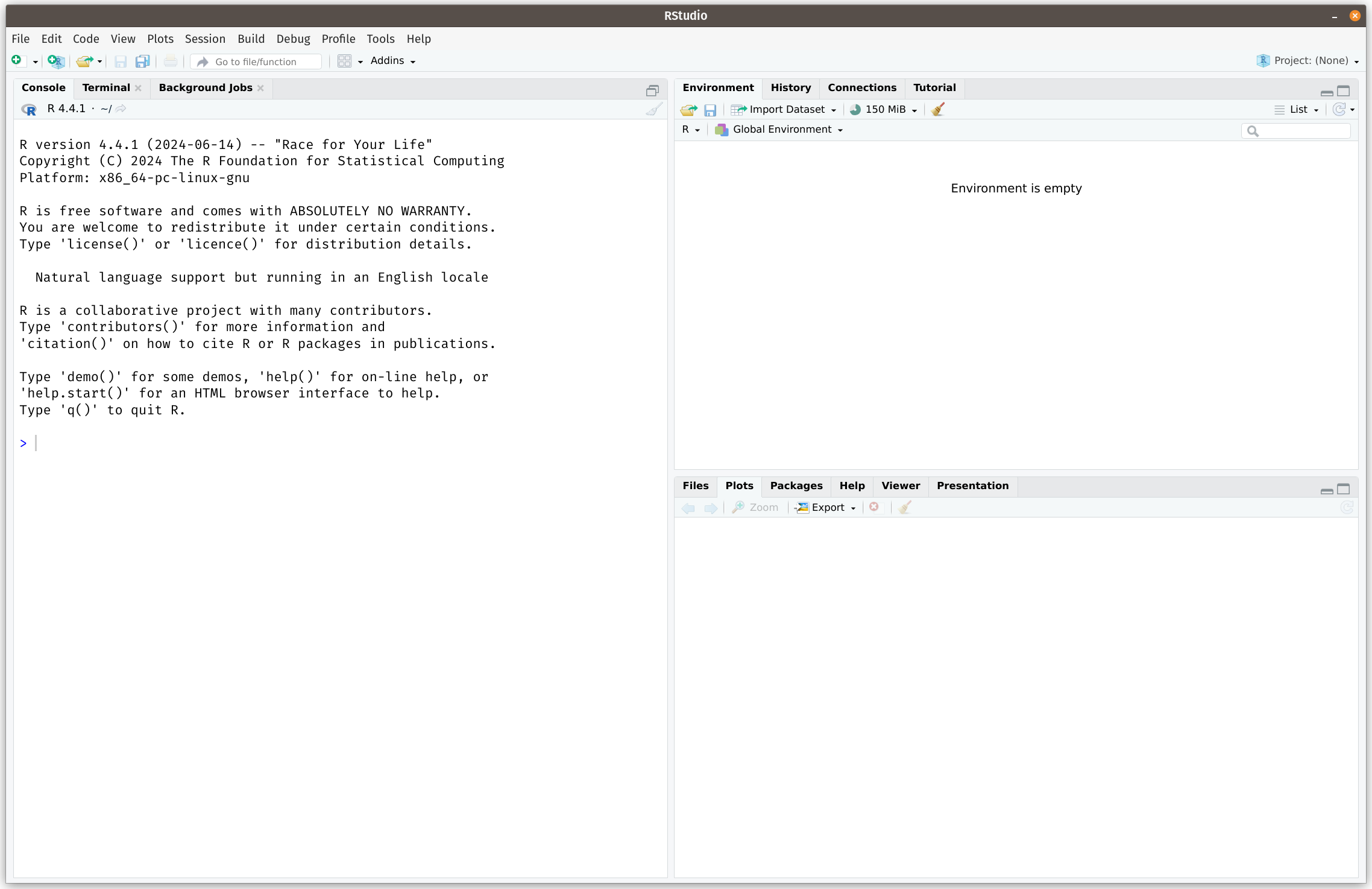
After these two steps, you can open RStudio on your system, as you would with any program. You should see something like this:
NoteNote for Windows users
While the installation steps above should be enough for most tasks, we also suggest that Windows users install RTools (click on the “Rtools44 installer” link at the middle of the page to get the .exe file). Rtools is needed on Windows to install some advanced packages, so it is a good idea to have it on your system.
That’s it for the installation! We also strongly recommend that you change a couple of RStudio’s default settings.1 You can change settings by clicking on Tools > Global Options in the menubar. Here are our recommendations:
General > Uncheck "Restore .RData into workspace at startup"General > Save workspace to .RData on Exit > Select "Never"Code > Check "Use native pipe operator"Tools > Global Options > Appearanceto change to a dark theme, if you want! Pros: better for night sessions, hacker vibes…
Working with RStudio Projects
One useful tool to organize your work in R is with RStudio Projects, which are files ending in .Rproj.
Why use RStudio Projects?
- Self-contained working directory: Opening an
.Rprojfile automatically sets R’s working directory to the project’s root folder. This means you can use clean relative file paths (e.g.,read_csv("data/my_data.csv")) instead of fragile, hard-coded machine paths likesetwd("C:/Users/name/Desktop/..."). - Portability and collaboration: Anyone who clones or unzips your project folder can run the code immediately without modifying file paths.
- Context preservation: RStudio remembers your open tabs, workspace history, and environment specifically for that project. This can be useful (though some would advise against being overreliant on this!).
Creating your own project from scratch
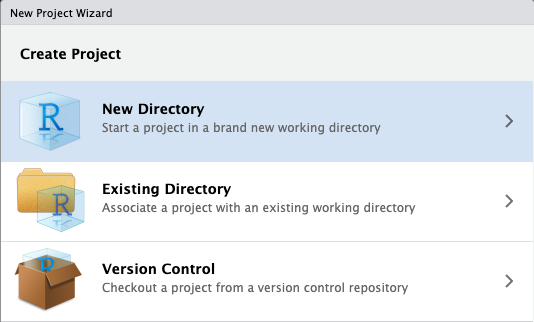
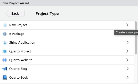
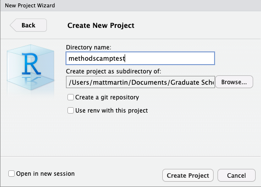
To create a new project in RStudio for your own coursework or research papers, click File > New Project, then follow the prompts:
TipRecommended Project Folder Structure
A standard, reproducible folder structure keeps your research organized and prevents accidental modification of raw data:
my_project/(Your root project folder containingmy_project.Rproj)code/(All.Rscripts and.qmdQuarto notebooks)data/raw/(Original, untouched raw data files—never edit these directly!)working/(Cleaned, processed datasets ready for modeling)
figures/(Exported plots and charts)tables/(Exported regression tables and summary statistics)
Using RStudio projects
When using an RStudio project, you should see its name in the top-right corner of RStudio, next to a light blue icon. You can check with R the folder in which your project operates:
- Now, as an example, let’s run the following commands in the script editor and save the files into the project directory.
library(tidyverse)

my_plot <- ggplot(mtcars, aes(wt, mpg)) +
    geom_point()

ggsave(
    plot = my_plot,
    filename = "plot_mtcars.pdf"
)

write_csv(mtcars, "mtcars.csv")
Quit RStudio and check out the folder associated with the project.
You should see the PDF file for the plot, the .csv file for the data, and the
.Rprojfile for the project itself.Double-click the
.Rprojfile to reopen the project and pick up where you left off! Everything you need should be ready to go.
Setting up for Methods Camp
All materials for Methods Camp are both on this website and available as RStudio projects for you to execute locally. An RStudio project is simply a folder where one keeps scripts, datasets, and other files needed for a data analysis project.
Below are RStudio projects for you to download, available as .zip compressed files. On MacOS, the file will be uncompressed automatically. On Windows, you should do Right click > Extract all.
- Download Part 1 of the class materials.
- Download Part 2 of the class materials.
- Download Part 3 of the class materials.
- Download Part 4 of the class materials.
Warning
Make sure to properly unzip the materials. Double-clicking the .zip file on most Windows systems will not unzip the folder—you must do Right click > Extract all.
You should now have a folder called methodscamp_part1/ on your computer. Navigate to the methodscamp_part1.Rproj file within it and open it. RStudio should open the project right away. You should see methodscamp_part1 on the top-right of RStudio—this indicates that you are working in our RStudio project.

Languages and Formats: R, Markdown, Quarto, and LaTeX
As you begin coding and writing research, you will encounter several different file formats and languages. Here is how they fit together:
- R Language & R Scripts (
.R):- R is the programming language executing calculations and statistical models.
- Plain
.Rscripts contain only code and comments (lines starting with#).
- Markdown (
.md):- A lightweight markup language used for formatting plain text with human-readable syntax (e.g.,
# Heading,**bold**,*italics*,[links](url)).
- A lightweight markup language used for formatting plain text with human-readable syntax (e.g.,
- Quarto Documents (
.qmd):- The modern successor to R Markdown. Quarto documents allow you to combine narrative Markdown text, executable R code chunks, and mathematical notation in a single document.
- This entire website is built using Quarto!
- LaTeX:
- A typesetting system used for mathematical and scientific publishing. In Quarto, you can write mathematical expressions enclosed in dollar signs (e.g.,
$\hat{\beta} = (X'X)^{-1}X'Y$), which render into beautiful math equations: \[\hat{\beta} = (X'X)^{-1}X'Y\]
- A typesetting system used for mathematical and scientific publishing. In Quarto, you can write mathematical expressions enclosed in dollar signs (e.g.,
Running Code vs. Rendering in Quarto
When working inside a Quarto document (.qmd), you have two ways to interact with code:
1. Interactive Execution (Running Chunks)
- You can run individual lines by pressing
Ctrl+Enter(Windows) /Cmd+Enter(Mac), or run an entire code chunk by clicking the green “Play” button in the top-right of the chunk (or pressingCtrl+Shift+Enter/Cmd+Shift+Enter). - This executes code directly in your active R console, saving variables to your current session memory.
The idea behind these settings (or at least the first two) is to force R to start from scratch with each new session. No lingering objects from previous coding sessions avoid misunderstandings and help with reproducibility!↩︎