2  Tidy data analysis I

The tidyverse is a suite of packages that streamline data analysis in R. After installing the tidyverse with install.packages("tidyverse") (see the previous module), you can load it with:

library(tidyverse)

── Attaching core tidyverse packages ──────────────────────── tidyverse 2.0.0 ──
✔ dplyr     1.1.4     ✔ readr     2.1.5
✔ forcats   1.0.0     ✔ stringr   1.5.1
✔ ggplot2   3.5.1     ✔ tibble    3.2.1
✔ lubridate 1.9.3     ✔ tidyr     1.3.1
✔ purrr     1.0.2     
── Conflicts ────────────────────────────────────────── tidyverse_conflicts() ──
✖ dplyr::filter() masks stats::filter()
✖ dplyr::lag()    masks stats::lag()
ℹ Use the conflicted package (<http://conflicted.r-lib.org/>) to force all conflicts to become errors

Tip

Upon loading, the tidyverse prints a message like the one above. Notice that multiple packages (the constituent elements of the “suite”) are actually loaded. For instance, dplyr and tidyr help with data wrangling and transformation, while ggplot2 allows us to draw plots. In most cases, one just loads the tidyverse and forgets about these details, as the constituent packages work together nicely.

Throughout this module, we will use tidyverse functions to load, wrangle, and visualize real data.

2.1 Loading data

Throughout this module we will work with a dataset of senators during the Trump presidency, which was adapted from FiveThirtyEight (2021).

We have stored the dataset in .csv format under the data/ subfolder. Loading it into R is simple (notice that we need to assign it to an object):

trump_scores <- read_csv("data/trump_scores_538.csv")

Rows: 122 Columns: 8
── Column specification ────────────────────────────────────────────────────────
Delimiter: ","
chr (4): bioguide, last_name, state, party
dbl (4): num_votes, agree, agree_pred, margin_trump

ℹ Use `spec()` to retrieve the full column specification for this data.
ℹ Specify the column types or set `show_col_types = FALSE` to quiet this message.

trump_scores

# A tibble: 122 × 8
   bioguide last_name  state party num_votes agree agree_pred margin_trump
   <chr>    <chr>      <chr> <chr>     <dbl> <dbl>      <dbl>        <dbl>
 1 A000360  Alexander  TN    R           118 0.890      0.856       26.0  
 2 B000575  Blunt      MO    R           128 0.906      0.787       18.6  
 3 B000944  Brown      OH    D           128 0.258      0.642        8.13 
 4 B001135  Burr       NC    R           121 0.893      0.560        3.66 
 5 B001230  Baldwin    WI    D           128 0.227      0.510        0.764
 6 B001236  Boozman    AR    R           129 0.915      0.851       26.9  
 7 B001243  Blackburn  TN    R           131 0.885      0.889       26.0  
 8 B001261  Barrasso   WY    R           129 0.891      0.895       46.3  
 9 B001267  Bennet     CO    D           121 0.273      0.417       -4.91 
10 B001277  Blumenthal CT    D           128 0.203      0.294      -13.6  
# ℹ 112 more rows

Let’s review the dataset’s columns:

• bioguide: A unique ID for each politician, from the Congress Bioguide.
• last_name
• state
• party
• num_votes: Number of votes for which data was available.
• agree: Proportion (0-1) of votes in which the senator voted in agreement with Trump.
• agree_pred: Predicted proportion of vote agreement, calculated using Trump’s margin (see next variable).
• margin_trump: Margin of victory (percentage points) of Trump in the senator’s state.

We can inspect our data by using the interface above. An alternative is to run the command View(trump_scores) or click on the object in RStudio’s environment panel (in the top-right section).

Do you have any questions about the data?

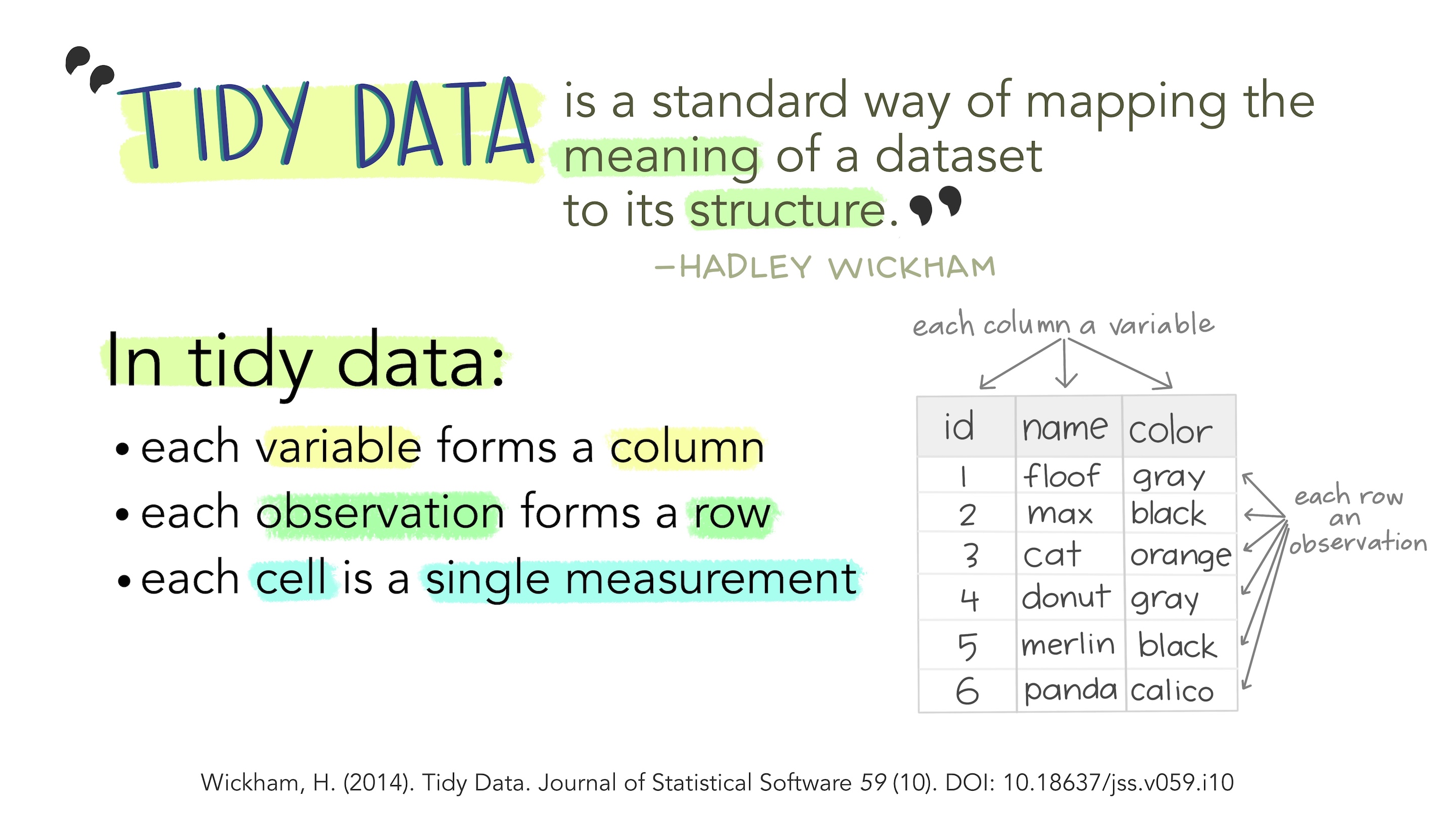
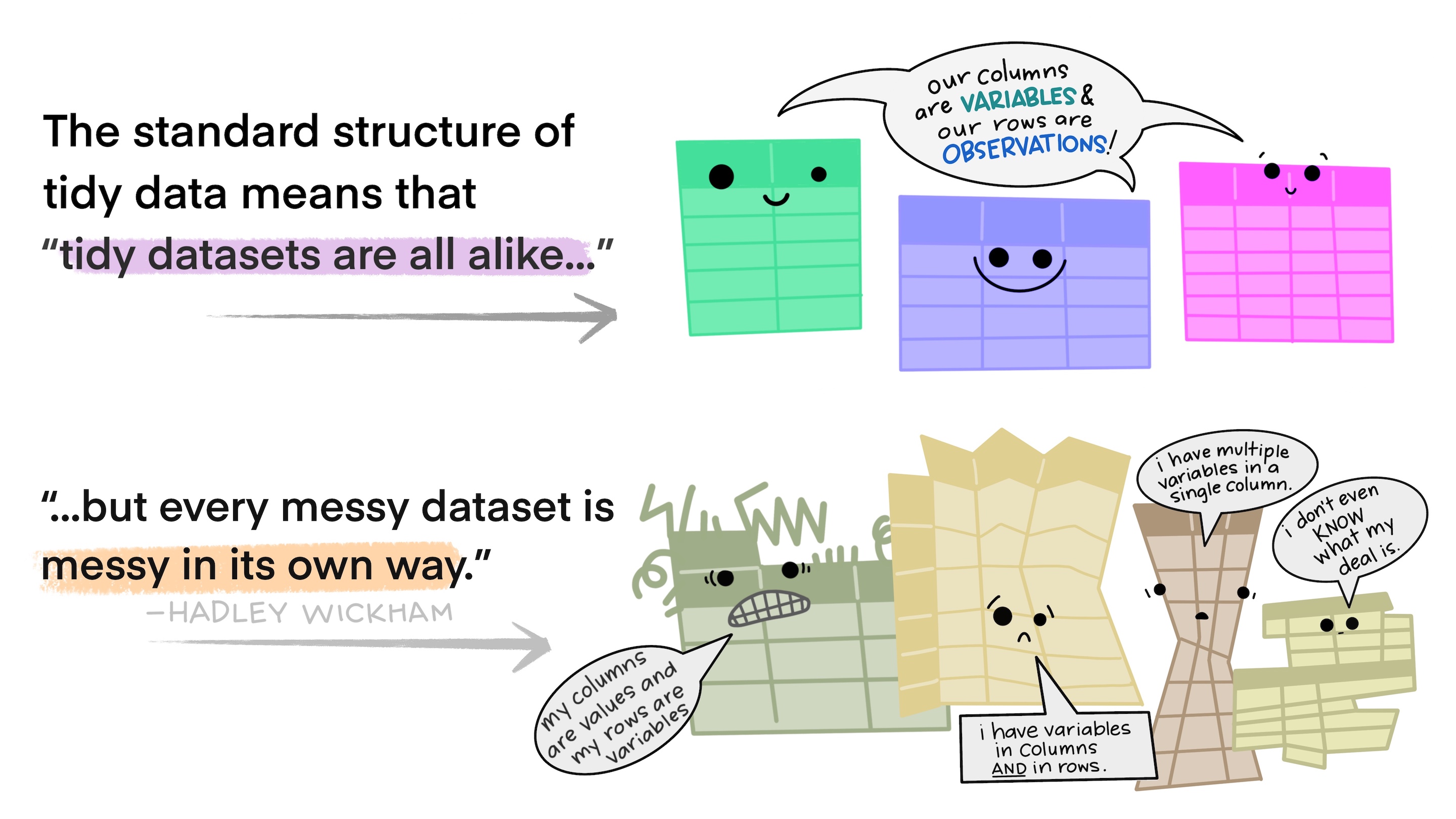
By the way, the tidyverse works amazingly with tidy data. If you can get your data to this format (and we will see ways to do this), your life will be much easier:

Source: Illustrations from the Openscapes blog Tidy Data for reproducibility, efficiency, and collaboration by Julia Lowndes and Allison Horst.

2.2 Wrangling data with dplyr

We often need to modify data to conduct our analyses, e.g., creating columns, filtering rows, etc. In the tidyverse, these operations are conducted with multiple verbs, which we will review now.

2.2.1 Selecting columns

We can select specific columns in our dataset with the select() function. All dplyr wrangling verbs take a data frame as their first argument—in this case, the columns we want to select are the other arguments.

select(trump_scores, last_name, party)

# A tibble: 122 × 2
   last_name  party
   <chr>      <chr>
 1 Alexander  R    
 2 Blunt      R    
 3 Brown      D    
 4 Burr       R    
 5 Baldwin    D    
 6 Boozman    R    
 7 Blackburn  R    
 8 Barrasso   R    
 9 Bennet     D    
10 Blumenthal D    
# ℹ 112 more rows

This is a good moment to talk about “pipes.” Notice how the code below produces the same output as the one above, but with a slightly different syntax. Pipes (|>) “kick” the object on the left of the pipe to the first argument of the function on the right. One can read pipes as “then,” so the code below can be read as “take trump_scores, then select the columns last_name and party.” Pipes are very useful to chain multiple operations, as we will see in a moment.

trump_scores |> 
  select(last_name, party)

# A tibble: 122 × 2
   last_name  party
   <chr>      <chr>
 1 Alexander  R    
 2 Blunt      R    
 3 Brown      D    
 4 Burr       R    
 5 Baldwin    D    
 6 Boozman    R    
 7 Blackburn  R    
 8 Barrasso   R    
 9 Bennet     D    
10 Blumenthal D    
# ℹ 112 more rows

Tip

You can insert a pipe with the Cmd/Ctrl + Shift + M shortcut. If you have not changed the default RStudio settings, an “old” pipe (%>%) might appear. While most of the functionality is the same, the |> “new” pipes are more readable and don’t need any extra packages (to use %>% you need the tidyverse or one of its packages). You can change this RStudio option in Tools > Global Options > Code > Use native pipe operator. Make sure to check the other suggested settings in our Setup module!

Going back to selecting columns, you can select ranges:

trump_scores |> 
  select(bioguide:party)

# A tibble: 122 × 4
   bioguide last_name  state party
   <chr>    <chr>      <chr> <chr>
 1 A000360  Alexander  TN    R    
 2 B000575  Blunt      MO    R    
 3 B000944  Brown      OH    D    
 4 B001135  Burr       NC    R    
 5 B001230  Baldwin    WI    D    
 6 B001236  Boozman    AR    R    
 7 B001243  Blackburn  TN    R    
 8 B001261  Barrasso   WY    R    
 9 B001267  Bennet     CO    D    
10 B001277  Blumenthal CT    D    
# ℹ 112 more rows

You can also deselect columns using a minus sign:

trump_scores |> 
  select(-last_name)

# A tibble: 122 × 7
   bioguide state party num_votes agree agree_pred margin_trump
   <chr>    <chr> <chr>     <dbl> <dbl>      <dbl>        <dbl>
 1 A000360  TN    R           118 0.890      0.856       26.0  
 2 B000575  MO    R           128 0.906      0.787       18.6  
 3 B000944  OH    D           128 0.258      0.642        8.13 
 4 B001135  NC    R           121 0.893      0.560        3.66 
 5 B001230  WI    D           128 0.227      0.510        0.764
 6 B001236  AR    R           129 0.915      0.851       26.9  
 7 B001243  TN    R           131 0.885      0.889       26.0  
 8 B001261  WY    R           129 0.891      0.895       46.3  
 9 B001267  CO    D           121 0.273      0.417       -4.91 
10 B001277  CT    D           128 0.203      0.294      -13.6  
# ℹ 112 more rows

And use a few helper functions, like matches():

trump_scores |> 
  select(last_name, matches("agree"))

# A tibble: 122 × 3
   last_name  agree agree_pred
   <chr>      <dbl>      <dbl>
 1 Alexander  0.890      0.856
 2 Blunt      0.906      0.787
 3 Brown      0.258      0.642
 4 Burr       0.893      0.560
 5 Baldwin    0.227      0.510
 6 Boozman    0.915      0.851
 7 Blackburn  0.885      0.889
 8 Barrasso   0.891      0.895
 9 Bennet     0.273      0.417
10 Blumenthal 0.203      0.294
# ℹ 112 more rows

Or everything(), which we usually use to reorder columns:

trump_scores |> 
  select(last_name, everything())

# A tibble: 122 × 8
   last_name  bioguide state party num_votes agree agree_pred margin_trump
   <chr>      <chr>    <chr> <chr>     <dbl> <dbl>      <dbl>        <dbl>
 1 Alexander  A000360  TN    R           118 0.890      0.856       26.0  
 2 Blunt      B000575  MO    R           128 0.906      0.787       18.6  
 3 Brown      B000944  OH    D           128 0.258      0.642        8.13 
 4 Burr       B001135  NC    R           121 0.893      0.560        3.66 
 5 Baldwin    B001230  WI    D           128 0.227      0.510        0.764
 6 Boozman    B001236  AR    R           129 0.915      0.851       26.9  
 7 Blackburn  B001243  TN    R           131 0.885      0.889       26.0  
 8 Barrasso   B001261  WY    R           129 0.891      0.895       46.3  
 9 Bennet     B001267  CO    D           121 0.273      0.417       -4.91 
10 Blumenthal B001277  CT    D           128 0.203      0.294      -13.6  
# ℹ 112 more rows

Tip

Notice that all these commands have not edited our existent objects—they have just printed the requested outputs to the screen. In order to modify objects, you need to use the assignment operator (<-). For example:

trump_scores_reduced <- trump_scores |> 
  select(last_name, matches("agree"))

trump_scores_reduced

# A tibble: 122 × 3
   last_name  agree agree_pred
   <chr>      <dbl>      <dbl>
 1 Alexander  0.890      0.856
 2 Blunt      0.906      0.787
 3 Brown      0.258      0.642
 4 Burr       0.893      0.560
 5 Baldwin    0.227      0.510
 6 Boozman    0.915      0.851
 7 Blackburn  0.885      0.889
 8 Barrasso   0.891      0.895
 9 Bennet     0.273      0.417
10 Blumenthal 0.203      0.294
# ℹ 112 more rows

Exercise

Select the variables last_name, party, num_votes, and agree from the data frame. Your code:

2.2.2 Renaming columns

We can use the rename() function to rename columns, with the syntax new_name = old_name. For example:

trump_scores |> 
  rename(prop_agree = agree, prop_agree_pred = agree_pred)

# A tibble: 122 × 8
   bioguide last_name  state party num_votes prop_agree prop_agree_pred
   <chr>    <chr>      <chr> <chr>     <dbl>      <dbl>           <dbl>
 1 A000360  Alexander  TN    R           118      0.890           0.856
 2 B000575  Blunt      MO    R           128      0.906           0.787
 3 B000944  Brown      OH    D           128      0.258           0.642
 4 B001135  Burr       NC    R           121      0.893           0.560
 5 B001230  Baldwin    WI    D           128      0.227           0.510
 6 B001236  Boozman    AR    R           129      0.915           0.851
 7 B001243  Blackburn  TN    R           131      0.885           0.889
 8 B001261  Barrasso   WY    R           129      0.891           0.895
 9 B001267  Bennet     CO    D           121      0.273           0.417
10 B001277  Blumenthal CT    D           128      0.203           0.294
# ℹ 112 more rows
# ℹ 1 more variable: margin_trump <dbl>

This is a good occasion to show how pipes allow us to chain operations. How do we read the following code out loud? (Remember that pipes are read as “then”).

trump_scores |> 
  select(last_name, matches("agree")) |> 
  rename(prop_agree = agree, prop_agree_pred = agree_pred)

# A tibble: 122 × 3
   last_name  prop_agree prop_agree_pred
   <chr>           <dbl>           <dbl>
 1 Alexander       0.890           0.856
 2 Blunt           0.906           0.787
 3 Brown           0.258           0.642
 4 Burr            0.893           0.560
 5 Baldwin         0.227           0.510
 6 Boozman         0.915           0.851
 7 Blackburn       0.885           0.889
 8 Barrasso        0.891           0.895
 9 Bennet          0.273           0.417
10 Blumenthal      0.203           0.294
# ℹ 112 more rows

2.2.3 Creating columns

It is common to want to create columns, based on existing ones. We can use mutate() to do so. For example, we could want our main variables of interest in terms of percentages instead of proportions:

trump_scores |> 
  select(last_name, agree, agree_pred) |> # select just for clarity
  mutate(pct_agree = 100 * agree,
         pct_agree_pred = 100 * agree_pred)

# A tibble: 122 × 5
   last_name  agree agree_pred pct_agree pct_agree_pred
   <chr>      <dbl>      <dbl>     <dbl>          <dbl>
 1 Alexander  0.890      0.856      89.0           85.6
 2 Blunt      0.906      0.787      90.6           78.7
 3 Brown      0.258      0.642      25.8           64.2
 4 Burr       0.893      0.560      89.3           56.0
 5 Baldwin    0.227      0.510      22.7           51.0
 6 Boozman    0.915      0.851      91.5           85.1
 7 Blackburn  0.885      0.889      88.5           88.9
 8 Barrasso   0.891      0.895      89.1           89.5
 9 Bennet     0.273      0.417      27.3           41.7
10 Blumenthal 0.203      0.294      20.3           29.4
# ℹ 112 more rows

We can also use multiple columns for creating a new one. For example, let’s retrieve the total number of votes in which the senator agreed with Trump:

trump_scores |> 
  select(last_name, num_votes, agree) |> # select just for clarity
  mutate(num_votes_agree = num_votes * agree)

# A tibble: 122 × 4
   last_name  num_votes agree num_votes_agree
   <chr>          <dbl> <dbl>           <dbl>
 1 Alexander        118 0.890           105  
 2 Blunt            128 0.906           116  
 3 Brown            128 0.258            33  
 4 Burr             121 0.893           108  
 5 Baldwin          128 0.227            29  
 6 Boozman          129 0.915           118  
 7 Blackburn        131 0.885           116  
 8 Barrasso         129 0.891           115  
 9 Bennet           121 0.273            33.0
10 Blumenthal       128 0.203            26  
# ℹ 112 more rows

2.2.4 Filtering rows

Another common operation is to filter rows based on logical conditions. We can do so with the filter() function. For example, we can filter to only get Democrats:

trump_scores |> 
  filter(party == "D")

# A tibble: 55 × 8
   bioguide last_name  state party num_votes agree agree_pred margin_trump
   <chr>    <chr>      <chr> <chr>     <dbl> <dbl>      <dbl>        <dbl>
 1 B000944  Brown      OH    D           128 0.258      0.642        8.13 
 2 B001230  Baldwin    WI    D           128 0.227      0.510        0.764
 3 B001267  Bennet     CO    D           121 0.273      0.417       -4.91 
 4 B001277  Blumenthal CT    D           128 0.203      0.294      -13.6  
 5 B001288  Booker     NJ    D           119 0.160      0.290      -14.1  
 6 C000127  Cantwell   WA    D           128 0.242      0.276      -15.5  
 7 C000141  Cardin     MD    D           128 0.25       0.209      -26.4  
 8 C000174  Carper     DE    D           129 0.295      0.318      -11.4  
 9 C001070  Casey      PA    D           129 0.287      0.508        0.724
10 C001088  Coons      DE    D           128 0.289      0.319      -11.4  
# ℹ 45 more rows

Notice that == here is a logical operator, read as “is equal to.” So our full chain of operations says the following: take trump_scores, then filter it to get rows where party is equal to “D”.

There are other logical operators:

Logical operator	Meaning
==	“is equal to”
!=	“is not equal to”
>	“is greater than”
<	“is less than”
>=	“is greater than or equal to”
<=	“is less than or equal to”
%in%	“is contained in”
&	“and” (intersection)
|	“or” (union)

Let’s see a couple of other examples.

trump_scores |> 
  filter(agree > 0.5)

# A tibble: 69 × 8
   bioguide last_name state party num_votes agree agree_pred margin_trump
   <chr>    <chr>     <chr> <chr>     <dbl> <dbl>      <dbl>        <dbl>
 1 A000360  Alexander TN    R           118 0.890      0.856        26.0 
 2 B000575  Blunt     MO    R           128 0.906      0.787        18.6 
 3 B001135  Burr      NC    R           121 0.893      0.560         3.66
 4 B001236  Boozman   AR    R           129 0.915      0.851        26.9 
 5 B001243  Blackburn TN    R           131 0.885      0.889        26.0 
 6 B001261  Barrasso  WY    R           129 0.891      0.895        46.3 
 7 B001310  Braun     IN    R            44 0.909      0.713        19.2 
 8 C000567  Cochran   MS    R            68 0.971      0.830        17.8 
 9 C000880  Crapo     ID    R           125 0.904      0.870        31.8 
10 C001035  Collins   ME    R           129 0.651      0.441        -2.96
# ℹ 59 more rows

trump_scores |> 
  filter(state %in% c("CA", "TX"))

# A tibble: 4 × 8
  bioguide last_name state party num_votes agree agree_pred margin_trump
  <chr>    <chr>     <chr> <chr>     <dbl> <dbl>      <dbl>        <dbl>
1 C001056  Cornyn    TX    R           129 0.922      0.659         9.00
2 C001098  Cruz      TX    R           126 0.921      0.663         9.00
3 F000062  Feinstein CA    D           128 0.242      0.201       -30.1 
4 H001075  Harris    CA    D           116 0.164      0.209       -30.1 

trump_scores |> 
  filter(state == "WV" & party == "D")

# A tibble: 1 × 8
  bioguide last_name state party num_votes agree agree_pred margin_trump
  <chr>    <chr>     <chr> <chr>     <dbl> <dbl>      <dbl>        <dbl>
1 M001183  Manchin   WV    D           129 0.504      0.893         42.2

Exercise

1. Add a new column to the data frame, called diff_agree, which subtracts agree and agree_pred. How would you create abs_diff_agree, defined as the absolute value of diff_agree? Your code:

2. Filter the data frame to only get senators for which we have information on fewer than (or equal to) five votes. Your code:

3. Filter the data frame to only get Democrats who agreed with Trump in at least 30% of votes. Your code:

2.2.5 Ordering rows

The arrange() function allows us to order rows according to values. For example, let’s order based on the agree variable:

trump_scores |> 
  arrange(agree)

# A tibble: 122 × 8
   bioguide last_name    state party num_votes agree agree_pred margin_trump
   <chr>    <chr>        <chr> <chr>     <dbl> <dbl>      <dbl>        <dbl>
 1 H000273  Hickenlooper CO    D             2 0         0.0302        -4.91
 2 H000601  Hagerty      TN    R             2 0         0.115         26.0 
 3 L000570  Luján        NM    D           186 0.124     0.243         -8.21
 4 G000555  Gillibrand   NY    D           121 0.124     0.242        -22.5 
 5 M001176  Merkley      OR    D           129 0.155     0.323        -11.0 
 6 W000817  Warren       MA    D           116 0.155     0.216        -27.2 
 7 B001288  Booker       NJ    D           119 0.160     0.290        -14.1 
 8 S000033  Sanders      VT    D           112 0.161     0.221        -26.4 
 9 H001075  Harris       CA    D           116 0.164     0.209        -30.1 
10 M000133  Markey       MA    D           127 0.165     0.213        -27.2 
# ℹ 112 more rows

Maybe we only want senators with more than a few data points. Remember that we can chain operations:

trump_scores |> 
  filter(num_votes >= 10) |> 
  arrange(agree)

# A tibble: 115 × 8
   bioguide last_name  state party num_votes agree agree_pred margin_trump
   <chr>    <chr>      <chr> <chr>     <dbl> <dbl>      <dbl>        <dbl>
 1 L000570  Luján      NM    D           186 0.124      0.243        -8.21
 2 G000555  Gillibrand NY    D           121 0.124      0.242       -22.5 
 3 M001176  Merkley    OR    D           129 0.155      0.323       -11.0 
 4 W000817  Warren     MA    D           116 0.155      0.216       -27.2 
 5 B001288  Booker     NJ    D           119 0.160      0.290       -14.1 
 6 S000033  Sanders    VT    D           112 0.161      0.221       -26.4 
 7 H001075  Harris     CA    D           116 0.164      0.209       -30.1 
 8 M000133  Markey     MA    D           127 0.165      0.213       -27.2 
 9 W000779  Wyden      OR    D           129 0.186      0.323       -11.0 
10 B001277  Blumenthal CT    D           128 0.203      0.294       -13.6 
# ℹ 105 more rows

By default, arrange() uses increasing order (like sort()). To use decreasing order, add a minus sign:

trump_scores |> 
  filter(num_votes >= 10) |> 
  arrange(-agree)

# A tibble: 115 × 8
   bioguide last_name state party num_votes agree agree_pred margin_trump
   <chr>    <chr>     <chr> <chr>     <dbl> <dbl>      <dbl>        <dbl>
 1 M001198  Marshall  KS    R           183 0.973      0.933        20.6 
 2 C000567  Cochran   MS    R            68 0.971      0.830        17.8 
 3 H000338  Hatch     UT    R            84 0.964      0.825        18.1 
 4 M001197  McSally   AZ    R           136 0.949      0.562         3.55
 5 P000612  Perdue    GA    R           119 0.941      0.606         5.16
 6 C001096  Cramer    ND    R           135 0.941      0.908        35.7 
 7 R000307  Roberts   KS    R           127 0.937      0.818        20.6 
 8 C001056  Cornyn    TX    R           129 0.922      0.659         9.00
 9 H001061  Hoeven    ND    R           129 0.922      0.883        35.7 
10 C001047  Capito    WV    R           127 0.921      0.896        42.2 
# ℹ 105 more rows

You can also order rows by more than one variable. What this does is to order by the first variable, and resolve any ties by ordering by the second variable (and so forth if you have more than two ordering variables). For example, let’s first order our data frame by party, and then within party order by agreement with Trump:

trump_scores |> 
  filter(num_votes >= 10) |> 
  arrange(party, agree)

# A tibble: 115 × 8
   bioguide last_name  state party num_votes agree agree_pred margin_trump
   <chr>    <chr>      <chr> <chr>     <dbl> <dbl>      <dbl>        <dbl>
 1 L000570  Luján      NM    D           186 0.124      0.243        -8.21
 2 G000555  Gillibrand NY    D           121 0.124      0.242       -22.5 
 3 M001176  Merkley    OR    D           129 0.155      0.323       -11.0 
 4 W000817  Warren     MA    D           116 0.155      0.216       -27.2 
 5 B001288  Booker     NJ    D           119 0.160      0.290       -14.1 
 6 S000033  Sanders    VT    D           112 0.161      0.221       -26.4 
 7 H001075  Harris     CA    D           116 0.164      0.209       -30.1 
 8 M000133  Markey     MA    D           127 0.165      0.213       -27.2 
 9 W000779  Wyden      OR    D           129 0.186      0.323       -11.0 
10 B001277  Blumenthal CT    D           128 0.203      0.294       -13.6 
# ℹ 105 more rows

Exercise

Arrange the data by diff_pred, the difference between agreement and predicted agreement with Trump. (You should have code on how to create this variable from the last exercise). Your code:

2.2.6 Summarizing data

dplyr makes summarizing data a breeze using the summarize() function:

trump_scores |> 
  summarize(mean_agree = mean(agree),
            mean_agree_pred = mean(agree_pred))

# A tibble: 1 × 2
  mean_agree mean_agree_pred
       <dbl>           <dbl>
1      0.592           0.572

To make summaries, we can use any function that takes a vector and returns one value. Another example:

trump_scores |> 
  filter(num_votes >= 5) |> # to filter out senators with few data points
  summarize(max_agree = max(agree),
            min_agree = min(agree))

# A tibble: 1 × 2
  max_agree min_agree
      <dbl>     <dbl>
1         1     0.124

Grouped summaries allow us to disaggregate summaries according to other variables (usually categorical):

trump_scores |> 
  filter(num_votes >= 5) |> # to filter out senators with few data points
  summarize(mean_agree = mean(agree),
            max_agree = max(agree),
            min_agree = min(agree),
            .by = party) # to group by party

# A tibble: 2 × 4
  party mean_agree max_agree min_agree
  <chr>      <dbl>     <dbl>     <dbl>
1 R          0.876     1         0.651
2 D          0.272     0.548     0.124

Exercise

Obtain the maximum absolute difference in agreement with Trump (the abs_diff_agree variable from before) for each party.

2.2.7 Overview

Function	Purpose
select()	Select columns
rename()	Rename columns
mutate()	Creating columns
filter()	Filtering rows
arrange()	Ordering rows
summarize()	Summarizing data
summarize(…, .by = )	Summarizing data (by groups)

2.3 Visualizing data with ggplot2

ggplot2 is the package in charge of data visualization in the tidyverse. It is extremely flexible and allows us to draw bar plots, box plots, histograms, scatter plots, and many other types of plots (see examples at R Charts).

Throughout this module we will use a subset of our data frame, which only includes senators with more than a few data points:

trump_scores_ss <- trump_scores |> 
  filter(num_votes >= 10)

The ggplot2 syntax provides a unifying interface (the “grammar of graphics” or “gg”) for drawing all different types of plots. One draws plots by adding different “layers,” and the core code always includes the following:

• A ggplot() command with a data = argument specifying a data frame and a mapping = aes() argument specifying “aesthetic mappings,” i.e., how we want to use the columns in the data frame in the plot (for example, in the x-axis, as color, etc.).

• “geoms,” such as geom_bar() or geom_point(), specifying what to draw on the plot.

So all ggplot2 commands will have at least three elements: data, aesthetic mappings, and geoms.

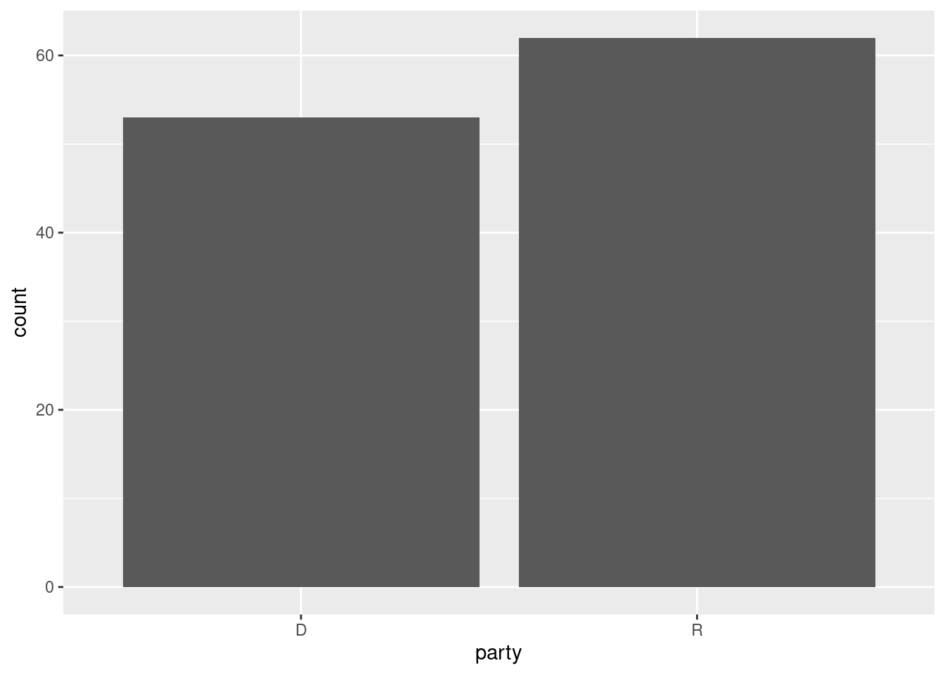
2.3.1 Univariate plots: categorical

Let’s see an example of a bar plot with a categorical variable:

ggplot(data = trump_scores_ss, mapping = aes(x = party)) +
  geom_bar()

Tip

As with any other function, we can drop the argument names if we specify the argument values in order. This is common in ggplot2 code:

ggplot(trump_scores_ss, aes(x = party)) +
  geom_bar()

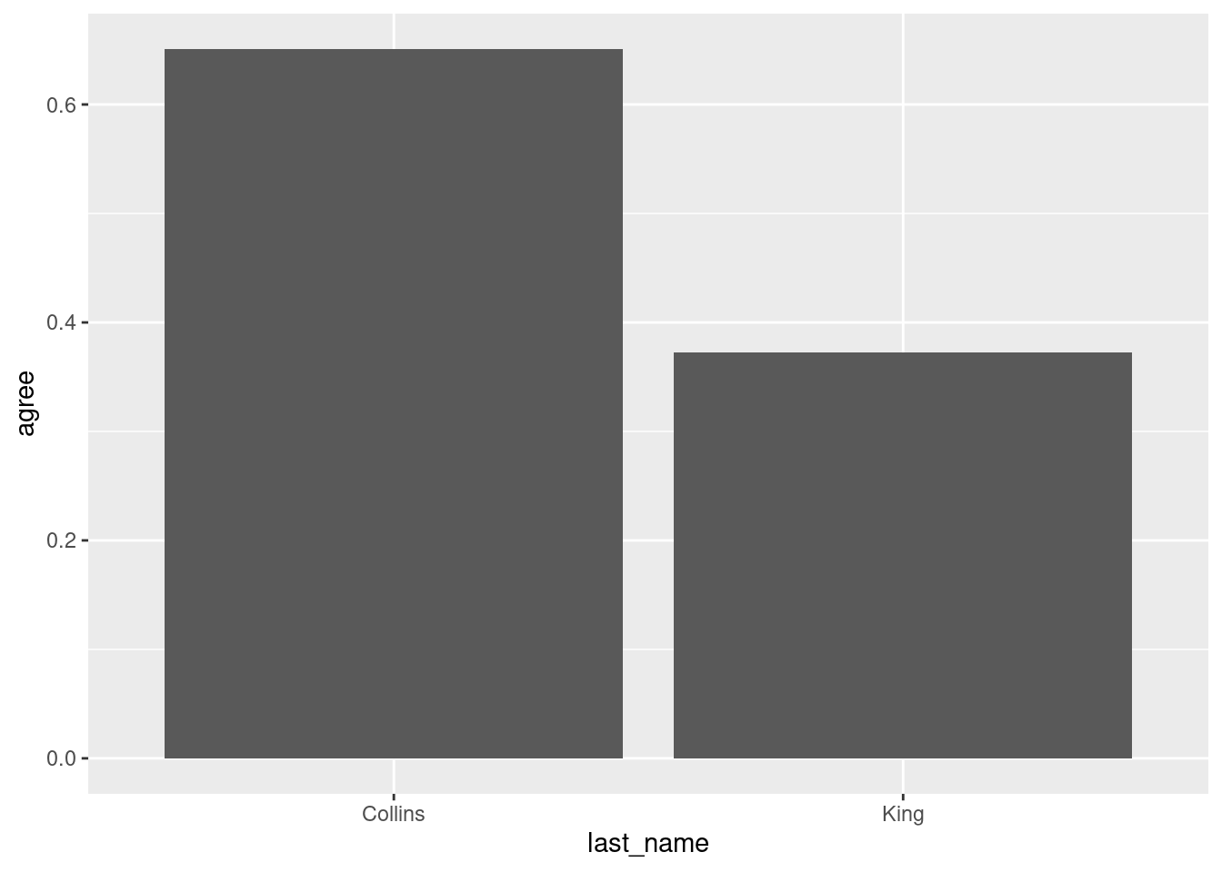
Notice how geom_bar() automatically computes the number of observations in each category for us. Sometimes we want to use numbers in our data frame as part of a bar plot. Here we can use the geom_col() geom specifying both x and y aesthetic mappings, in which is sometimes called a “column plot:”

ggplot(trump_scores_ss |> filter(state == "ME"),
       aes(x = last_name, y = agree)) +
  geom_col()

Exercise

Draw a column plot with the agreement with Trump of Bernie Sanders and Ted Cruz. What happens if you use last_name as the y aesthetic mapping and agree in the x aesthetic mapping? Your code:

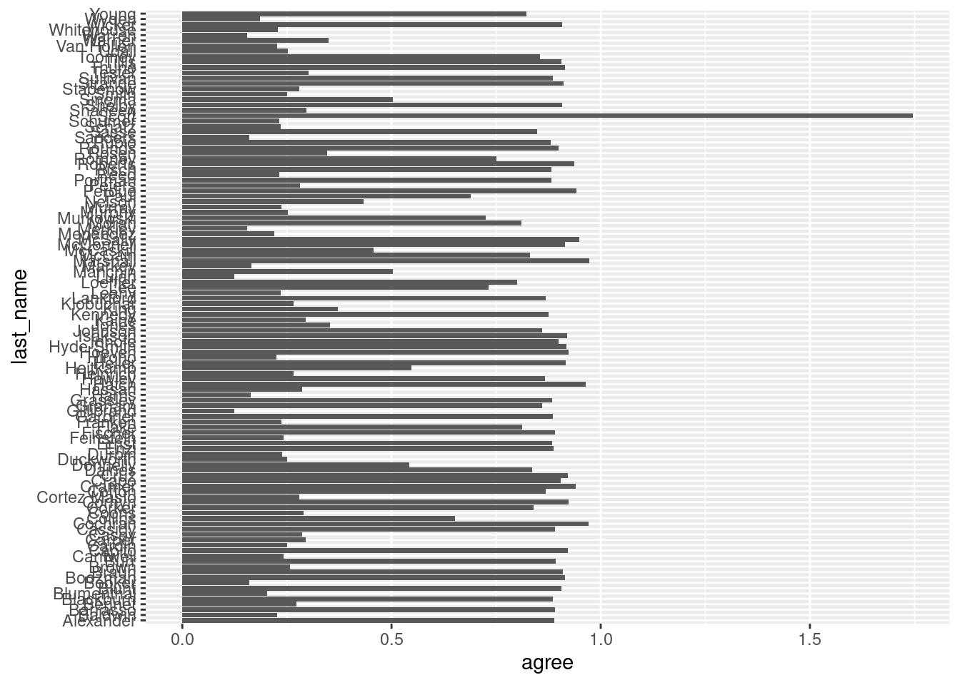
A common use of geom_col() is to create “ranking plots.” For example, who are the senators with highest agreement with Trump? We can start with something like this:

ggplot(trump_scores_ss,
       aes(x = agree, y = last_name)) +
  geom_col()

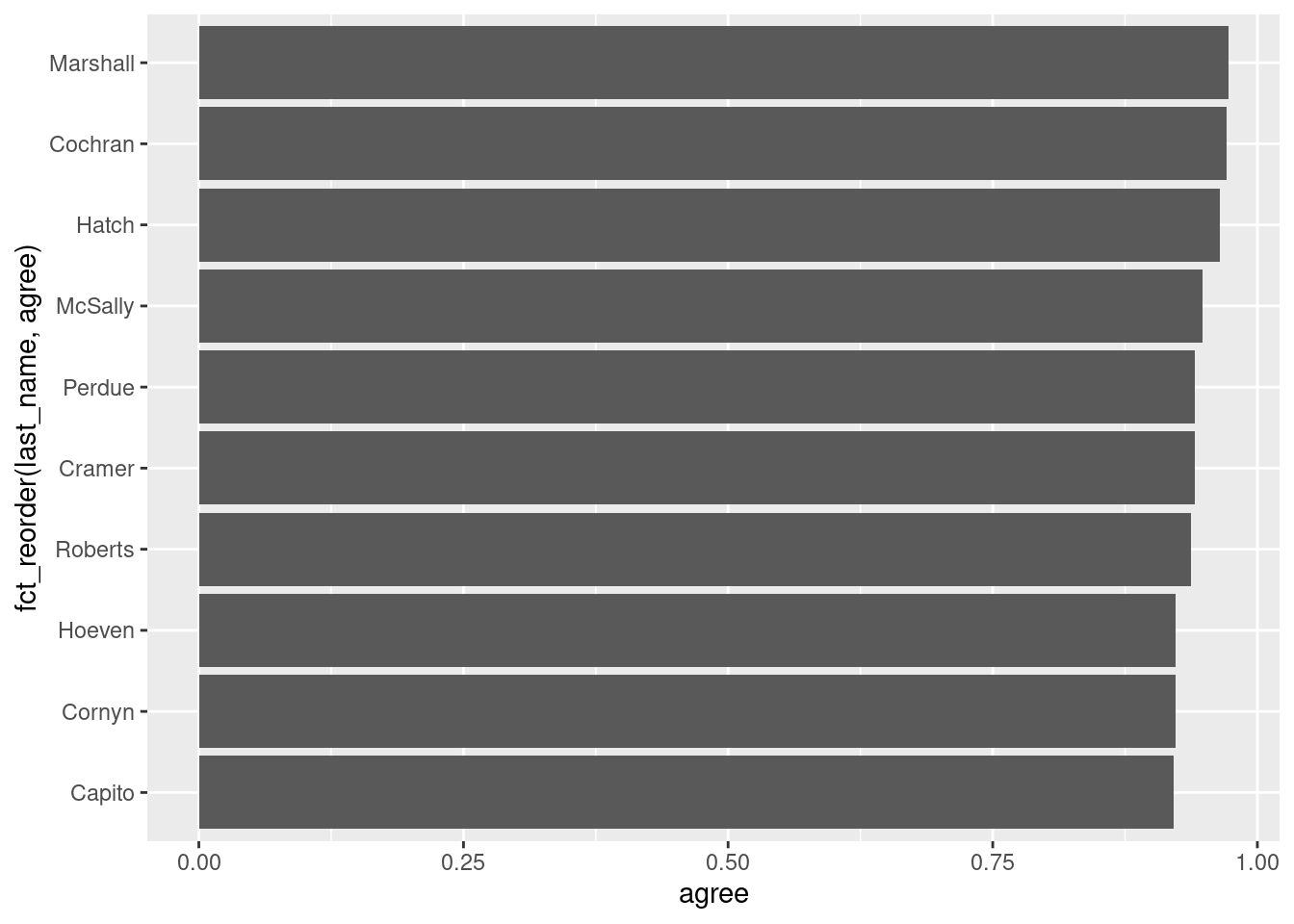
We might want to (1) select the top 10 observations and (2) order the bars according to the agree values. We can do these operations with slice_max() and fct_reorder(), as shown below:

ggplot(trump_scores_ss |> slice_max(agree, n = 10),
       aes(x = agree, y = fct_reorder(last_name, agree))) +
  geom_col()

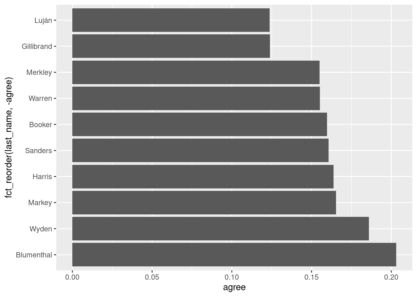
We can also plot the senators with the lowest agreement with Trump using slice_min() and fct_reorder() with a minus sign in the ordering variable:

ggplot(trump_scores_ss |> slice_min(agree, n = 10),
       aes(x = agree, y = fct_reorder(last_name, -agree))) +
  geom_col()

2.3.2 Univariate plots: numerical

We can draw a histogram with geom_histogram():

ggplot(trump_scores_ss, aes(x = agree)) +
  geom_histogram()

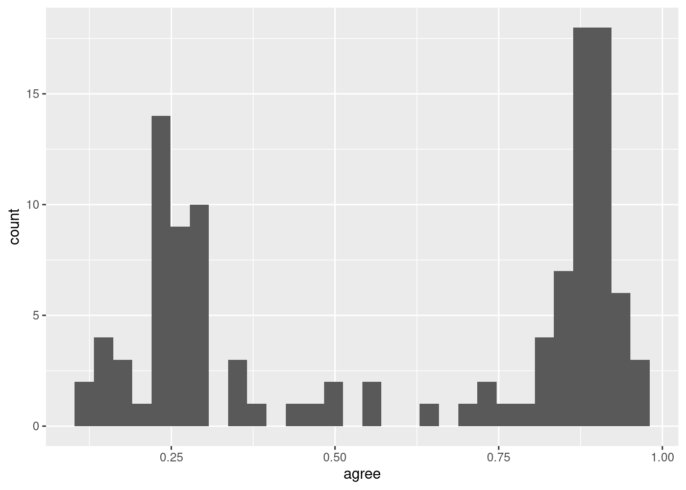
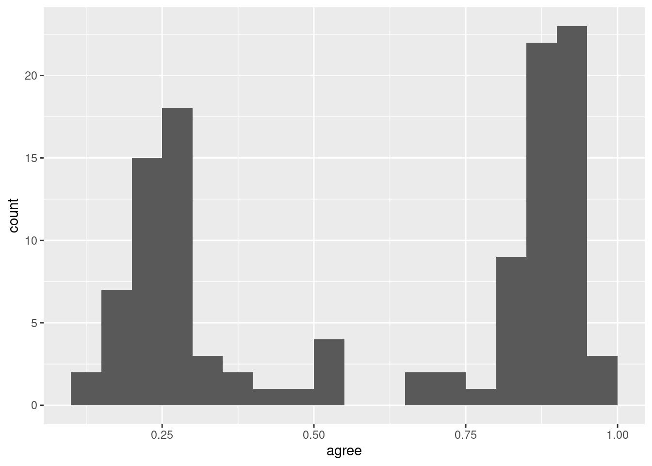
`stat_bin()` using `bins = 30`. Pick better value with `binwidth`.

Notice the warning message above. It’s telling us that, by default, geom_histogram() will draw 30 bins. Sometimes we want to modify this behavior. The following code has some common options for geom_histogram() and their explanations:

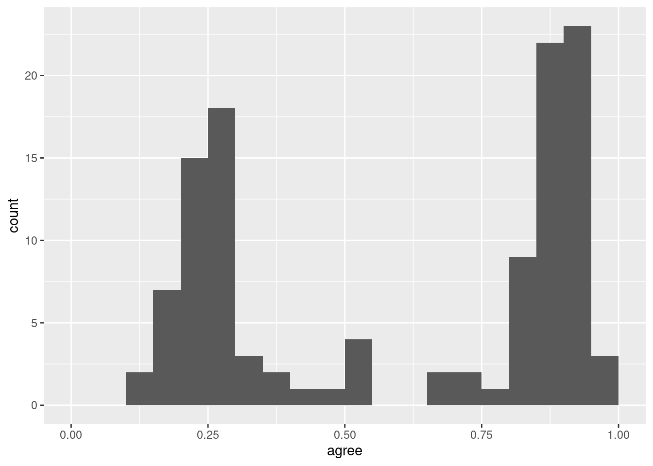
ggplot(trump_scores_ss, aes(x = agree)) +
  geom_histogram(binwidth = 0.05,   # draw bins every 0.05 jumps in x
                 boundary = 0,      # don't shift bins to integers
                 closed   = "left") # close bins on the left

Sometimes we want to manually alter a scale. This is accomplished with the scale_*() family of ggplot2 functions. Here we use the scale_x_continuous() function to make the x-axis go from 0 to 1:

ggplot(trump_scores_ss, aes(x = agree)) +
  geom_histogram(binwidth = 0.05, boundary = 0, closed   = "left") +   
  scale_x_continuous(limits = c(0, 1))

Adding the fill aesthetic mapping to a histogram will divide it according to a categorical variable. This is actually a bivariate plot!

ggplot(trump_scores_ss, aes(x = agree, fill = party)) +
  geom_histogram(binwidth = 0.05, boundary = 0, closed   = "left") +   
  scale_x_continuous(limits = c(0, 1)) +
  # change default colors:
  scale_fill_manual(values = c("D" = "blue", "R" = "red"))

2.3.3 Bivariate plots

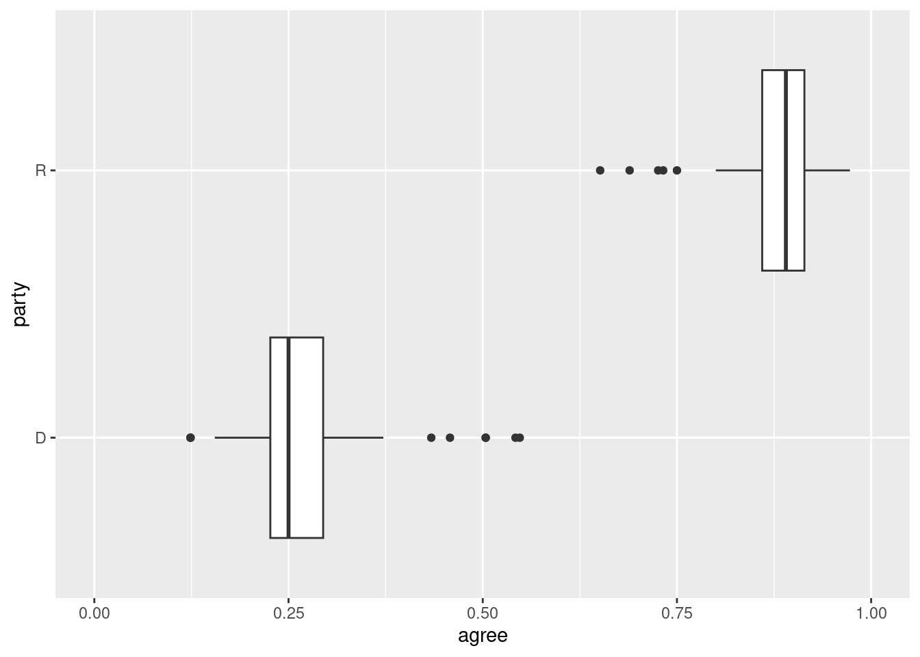
Another common bivariate plot for categorical and numerical variables is the grouped box plot:

ggplot(trump_scores_ss, aes(x = agree, y = party)) +
  geom_boxplot() +
  scale_x_continuous(limits = c(0, 1)) # same change as before

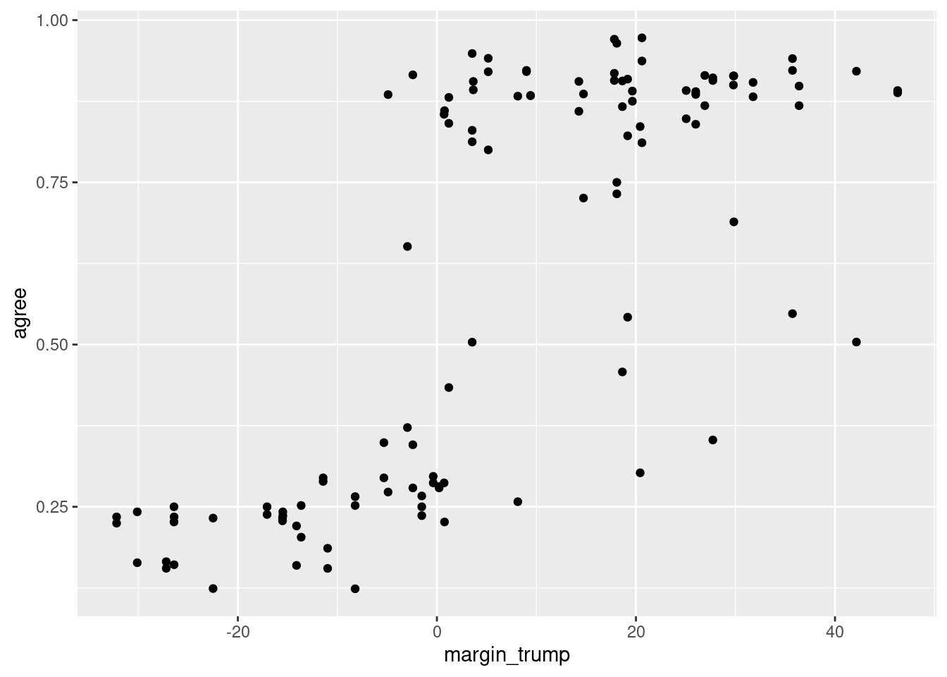
For bivariate plots of numerical variables, scatter plots are made with geom_point():

ggplot(trump_scores_ss, aes(x = margin_trump, y = agree)) +
  geom_point()

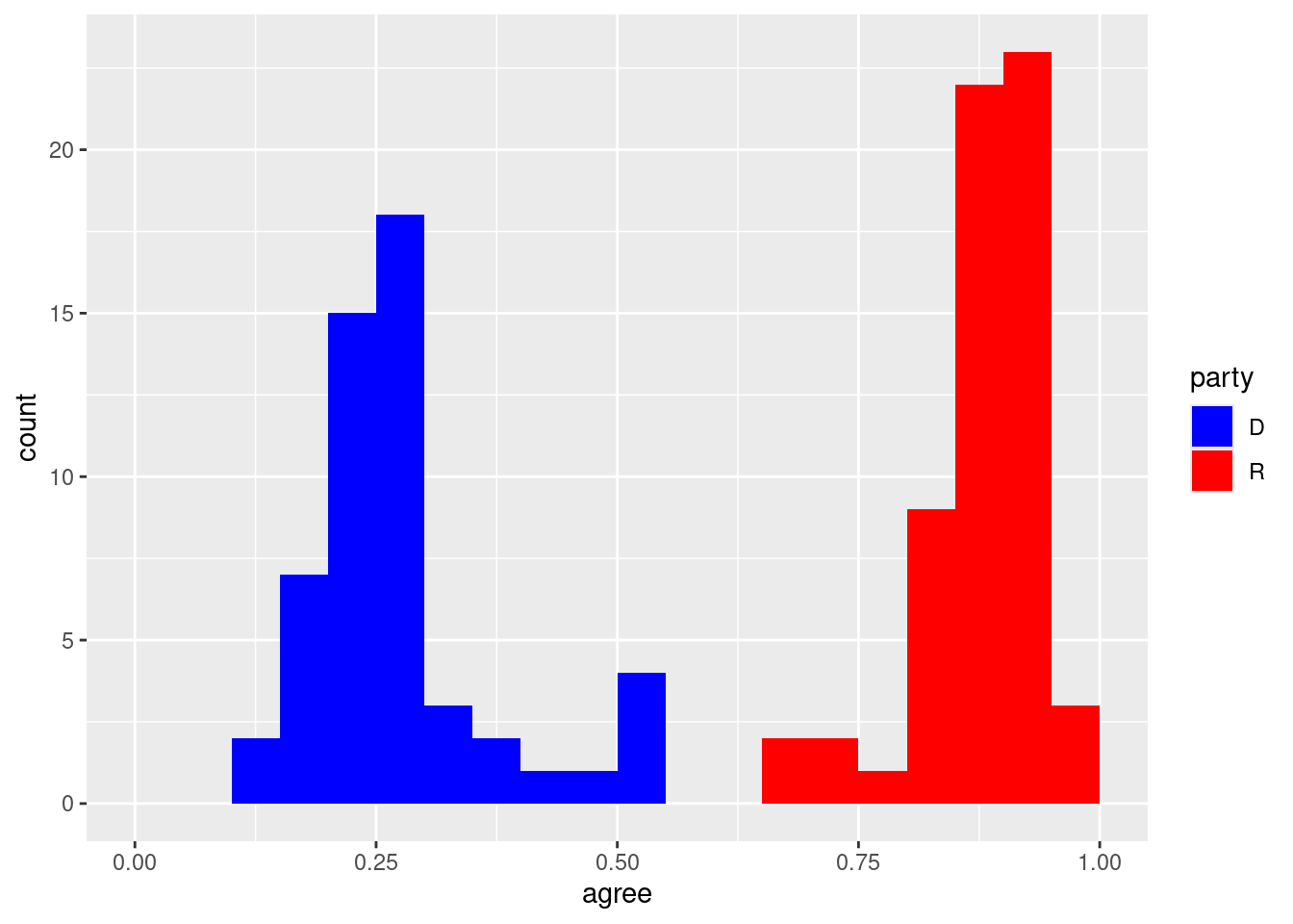
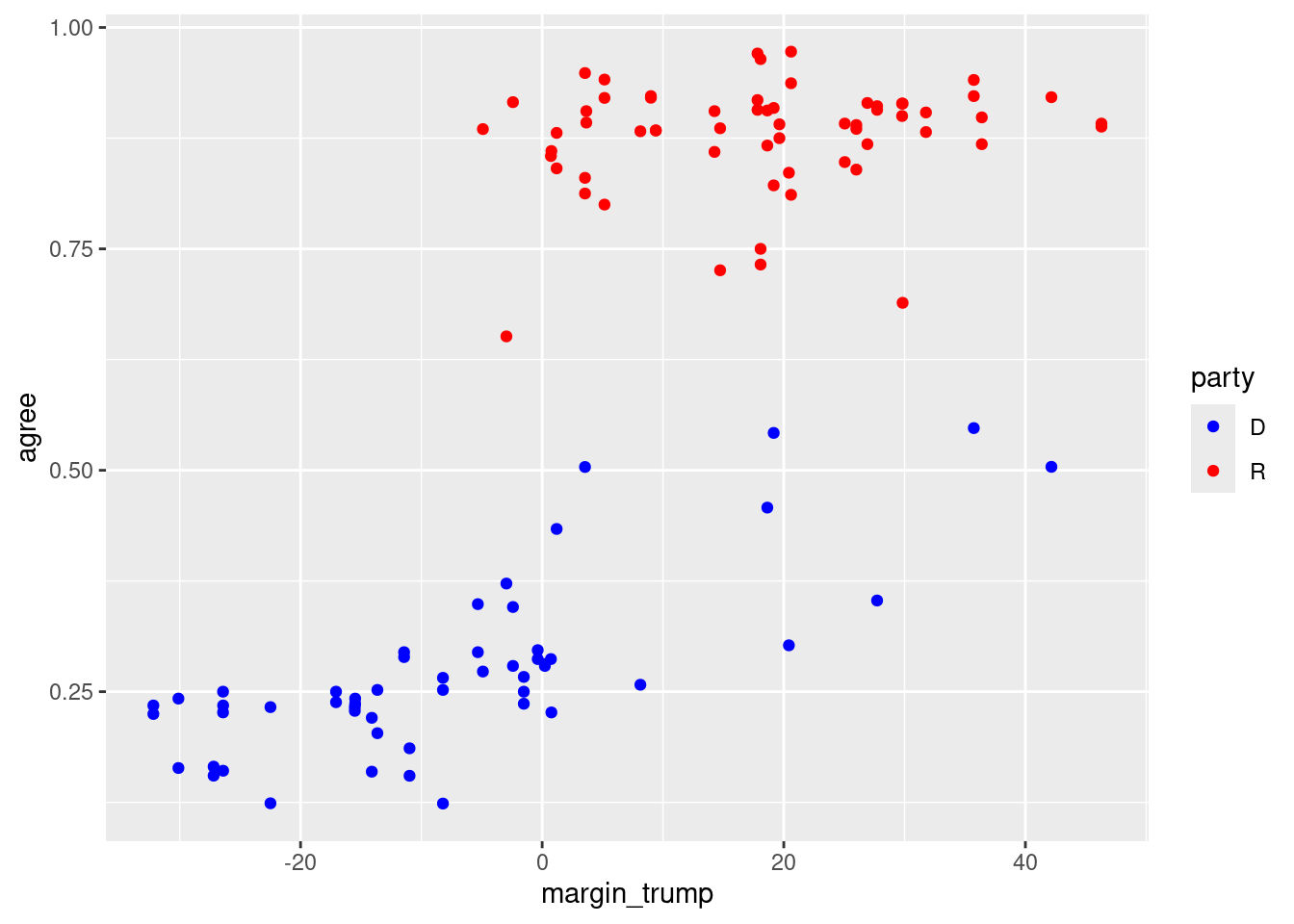
We can add the color aesthetic mapping to add a third variable:

ggplot(trump_scores_ss, aes(x = margin_trump, y = agree, color = party)) +
  geom_point() +
  scale_color_manual(values = c("D" = "blue", "R" = "red"))

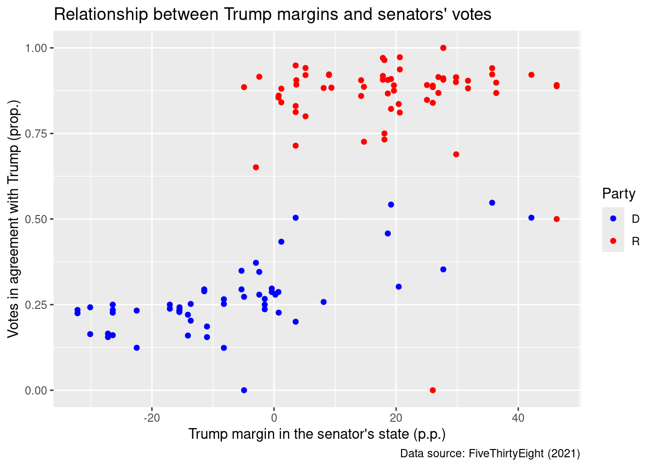
Let’s finish our plot with the labs() function, which allows us to add labels to our aesthetic mappings, as well as titles and notes:

ggplot(trump_scores, aes(x = margin_trump, y = agree, color = party)) +
  geom_point() +
  scale_color_manual(values = c("D" = "blue", "R" = "red")) +
  labs(x = "Trump margin in the senator's state (p.p.)",
       y = "Votes in agreement with Trump (prop.)",
       color = "Party",
       title = "Relationship between Trump margins and senators' votes",
       caption = "Data source: FiveThirtyEight (2021)")

We will review a few more customization options, including text labels and facets, in a subsequent module.

Arel-Bundock, Vincent, Nils Enevoldsen, and CJ Yetman. 2018. “Countrycode: An r Package to Convert Country Names and Country Codes.” Journal of Open Source Software 3 (28): 848. https://doi.org/10.21105/joss.00848.

Aronow, Peter M, and Benjamin T Miller. 2019. Foundations of Agnostic Statistics. Cambridge University Press.

Bank, World. 2023. “World Bank Open Data.” https://data.worldbank.org/.

Baydin, Atılım Günes, Barak A. Pearlmutter, Alexey Andreyevich Radul, and Jeffrey Mark Siskind. 2017. “Automatic Differentiation in Machine Learning: A Survey.” The Journal of Machine Learning Research 18 (1): 5595–5637.

Coppedge, Michael, John Gerring, Carl Henrik Knutsen, Staffan I. Lindberg, Jan Teorell, David Altman, Michael Bernhard, et al. 2022. “V-Dem Codebook V12.” Varieties of Democracy (V-Dem) Project. https://www.v-dem.net/dsarchive.html.

Dahlberg, Stefan, Aksen Sundström, Sören Holmberg, Bo Rothstein, Natalia Alvarado Pachon, Cem Mert Dalli, and Yente Meijers. 2023. “The Quality of Government Basic Dataset, Version Jan23.” University of Gothenburg: The Quality of Government Institute. https://www.gu.se/en/quality-government doi:10.18157/qogbasjan23.

FiveThirtyEight. 2021. “Tracking Congress In The Age Of Trump [Dataset].” https://projects.fivethirtyeight.com/congress-trump-score/.

Imai, Kosuke, and Nora Webb Williams. 2022. Quantitative Social Science: An Introduction in Tidyverse. Princeton; Oxford: Princeton University Press.

Moore, Will H., and David A. Siegel. 2013. A Mathematics Course for Political and Social Research. Princeton, NJ: Princeton University Pres.

Pontin, Jason. 2007. “Oppenheimer’s Ghost.” MIT Technology Review, October 15, 2007. https://www.technologyreview.com/2007/10/15/223531/oppenheimers-ghost-3/.

Robinson, David. 2020. Fuzzyjoin: Join Tables Together on Inexact Matching. https://github.com/dgrtwo/fuzzyjoin.

Rossi, Hugo. 1996. “Mathematics Is an Edifice, Not a Toolbox.” Notices of the AMS 43 (10): 1108.

Smith, Danny. 2020. Survey Research Datasets and R. https://socialresearchcentre.github.io/r_survey_datasets/.

U. S. Department of Agriculture [USDA], Agricultural Research Service. 2019. “Department of Agriculture Agricultural Research Service.” https://fdc.nal.usda.gov/.

Whittinghill, Dexter C, and Robert V Hogg. 2001. “A Little Uniform Density with Big Instructional Potential.” Journal of Statistics Education 9 (2).

Wickham, Hadley. 2014. “Tidy Data.” Journal of Statistical Software 59 (10). https://doi.org/10.18637/jss.v059.i10.

Wickham, Hadley, Danielle Navarro, and Thomas Lin Pedersen. 2023. Ggplot2: Elegant Graphics for Data Analysis. 3rd ed. https://ggplot2-book.org/.