Notice how in the data/ folder we have multiple versions of the same dataset (a subset of the QOG basic dataset): .csv (comma-separated values), .rds (R), .xlsx (Excel), .dta (Stata), and .sav (SPSS).
5.1.1 CSV and R data files
We can use the read_csv() and read_rds() functions from the tidyverse1 to read the .csv and .rds (R) data files:
Rows: 1085 Columns: 8
── Column specification ────────────────────────────────────────────────────────
Delimiter: ","
chr (4): cname, ccodealp, region, ht_colonial
dbl (4): year, wdi_pop, vdem_polyarchy, vdem_corr

ℹ Use `spec()` to retrieve the full column specification for this data.
ℹ Specify the column types or set `show_col_types = FALSE` to quiet this message.
For reading files from other software (Excel, Stata, or SPSS), we need to load additional packages. Luckily, they are automatically installed when one installs the tidyverse.
5.1.2 Excel data files
For Excel files (.xls or .xlsx files), the readxl package has a handy read_excel() function.
Useful arguments of the read_excel() function include sheet =, which reads particular sheets (specified via their positions or sheet names), and range =, which extracts a particular cell range (e.g., `A5:E25`).
5.1.3 Stata and SPSS data files
To load files from Stata (.dta) or SPSS (.spss), one needs the haven package and its properly-named read_stata() and read_spss() functions:
Datasets from Stata and SPSS can have additional properties, like variable labels and special types of missing values. To learn more about this, check out the “Labelled data” chapter from Danny Smith’s Survey Research Datasets and R(2020).
5.1.4 Our data for this session
We will rename one of our objects to qog:
qog <- qog_csvqog
# A tibble: 1,085 × 8
   cname      ccodealp  year region wdi_pop vdem_polyarchy vdem_corr ht_colonial
   <chr>      <chr>    <dbl> <chr>    <dbl>          <dbl>     <dbl> <chr>
 1 Antigua a… ATG       1990 Carib…   63328             NA        NA British
 2 Antigua a… ATG       1991 Carib…   63634             NA        NA British
 3 Antigua a… ATG       1992 Carib…   64659             NA        NA British
 4 Antigua a… ATG       1993 Carib…   65834             NA        NA British
 5 Antigua a… ATG       1994 Carib…   67072             NA        NA British
 6 Antigua a… ATG       1995 Carib…   68398             NA        NA British
 7 Antigua a… ATG       1996 Carib…   69798             NA        NA British
 8 Antigua a… ATG       1997 Carib…   71218             NA        NA British
 9 Antigua a… ATG       1998 Carib…   72572             NA        NA British
10 Antigua a… ATG       1999 Carib…   73821             NA        NA British
# ℹ 1,075 more rows
This dataset is a small sample of QOG, which contains data for countries in the Americas from 1990 to 2020. The observational unit is thus country-year. You can access the full codebook online. The variables are as follows:
Variable
Description
cname
Country name
ccodealp
Country code (ISO-3 character convention)
year
Year
region
Region (following legacy WDI convention). Added to QOG by us.
wdi_pop
Total population, from the World Development Indicators
vdem_polyarchy
V-Dem’s polyarchy index (electoral democracy)
vdem_corr
V-Dem’s corruption index
ht_colonial
Former colonial ruler
5.2 Recoding variables
Take a look at the ht_colonial variable. We can do a simple tabulation with count():
qog |>count(ht_colonial)
# A tibble: 6 × 2
  ht_colonial         n
  <chr>           <int>
1 British           372
2 Dutch              31
3 French             31
4 Never colonized    62
5 Portuguese         31
6 Spanish           558
Tip
Another common way to compute quick tabulations in R is with the table() function. Be aware that this takes a vector as the input:
table(qog$ht_colonial)
        British           Dutch          French Never colonized      Portuguese
            372              31              31              62              31
        Spanish
            558
We might want to recode this variable. For instance, we could create a dummy/binary variable for whether the country was a British colony. We can do this with if_else(), which works with logical conditions:
qog |># the arguments are condition, true (what to do if true), falsemutate(d_britishcol =if_else(ht_colonial =="British", 1, 0)) |>count(d_britishcol)
# A tibble: 2 × 2
  d_britishcol     n
         <dbl> <int>
1            0   713
2            1   372
Instead of a numeric classification (0 and 1), we could use characters:
# A tibble: 2 × 2
  cat_britishcol     n
  <chr>          <int>
1 British          372
2 Other            713
if_else() is great for binary recoding. But sometimes we want to create more than two categories. We can use case_when():
qog |># syntax is condition ~ valuemutate(cat_col =case_when( ht_colonial =="British"~"British", ht_colonial =="Spanish"~"Spanish", .default ="Other"# what to do in all other cases )) |>count(cat_col)
# A tibble: 3 × 2
  cat_col     n
  <chr>   <int>
1 British   372
2 Other     155
3 Spanish   558
The .default = argument in case_when() can also be used to leave the variable as-is for non-specified cases. For example, let’s combine Portuguese and Spanish colonies:
qog |># syntax is condition ~ valuemutate(cat_col =case_when( ht_colonial %in%c("Spanish", "Portuguese") ~"Spanish/Portuguese",.default = ht_colonial # what to do in all other cases )) |>count(cat_col)
# A tibble: 5 × 2
  cat_col                n
  <chr>              <int>
1 British              372
2 Dutch                 31
3 French                31
4 Never colonized       62
5 Spanish/Portuguese   589
NoteExercise
Create a dummy variable, d_large_pop, for whether the country-year has a population of more than 1 million. Then compute its mean. Your code:
Which countries are recorded as “Never colonized”? Change their values to other reasonable codings and compute a tabulation with count(). Your code:
5.3 Missing values
Missing values are commonplace in real datasets. In R, missing values are a special type of value in vectors, denoted as NA.
Warning
The special value NA is different from the character value “NA”. For example, notice that a numeric vector can have NAs, while it obviously cannot hold the character value “NA”:
c(5, 4.6, NA, 8)
[1] 5.0 4.6 NA 8.0
A quick way to check for missing values in small datasets is with the summary() function:
summary(qog)
    cname             ccodealp              year         region
 Length:1085        Length:1085        Min.   :1990   Length:1085
 Class :character   Class :character   1st Qu.:1997   Class :character
 Mode  :character   Mode  :character   Median :2005   Mode  :character
                                       Mean   :2005
                                       3rd Qu.:2013
                                       Max.   :2020

    wdi_pop          vdem_polyarchy     vdem_corr      ht_colonial
 Min.   :    40542   Min.   :0.0710   Min.   :0.0260   Length:1085
 1st Qu.:   389131   1st Qu.:0.5570   1st Qu.:0.1890   Class :character
 Median :  5687744   Median :0.7030   Median :0.5550   Mode  :character
 Mean   : 25004057   Mean   :0.6569   Mean   :0.4922
 3rd Qu.: 16195902   3rd Qu.:0.8030   3rd Qu.:0.7540
 Max.   :331501080   Max.   :0.9160   Max.   :0.9630
                     NA's   :248      NA's   :248
Notice that we have missingness in the vdem_polyarchy and vdem_corr variables. We might want to filter the dataset to see which observations are in this situation:
qog |>filter(vdem_polyarchy ==NA| vdem_corr ==NA)
# A tibble: 0 × 8
# ℹ 8 variables: cname <chr>, ccodealp <chr>, year <dbl>, region <chr>,
#   wdi_pop <dbl>, vdem_polyarchy <dbl>, vdem_corr <dbl>, ht_colonial <chr>
But the code above doesn’t work! To refer to missing values in logical conditions, we cannot use == NA. Instead, we need to use the is.na() function:
# A tibble: 248 × 8
   cname      ccodealp  year region wdi_pop vdem_polyarchy vdem_corr ht_colonial
   <chr>      <chr>    <dbl> <chr>    <dbl>          <dbl>     <dbl> <chr>
 1 Antigua a… ATG       1990 Carib…   63328             NA        NA British
 2 Antigua a… ATG       1991 Carib…   63634             NA        NA British
 3 Antigua a… ATG       1992 Carib…   64659             NA        NA British
 4 Antigua a… ATG       1993 Carib…   65834             NA        NA British
 5 Antigua a… ATG       1994 Carib…   67072             NA        NA British
 6 Antigua a… ATG       1995 Carib…   68398             NA        NA British
 7 Antigua a… ATG       1996 Carib…   69798             NA        NA British
 8 Antigua a… ATG       1997 Carib…   71218             NA        NA British
 9 Antigua a… ATG       1998 Carib…   72572             NA        NA British
10 Antigua a… ATG       1999 Carib…   73821             NA        NA British
# ℹ 238 more rows
Notice that, in most R functions, missing values are “contagious.” This means that any missing value will contaminate the operation and carry over to the results. For example:
Sometimes we’d like to perform our operations even in the presence of missing values, simply excluding them. Most basic R functions have an na.rm = argument to do this:
# A tibble: 1 × 1
  mean_vdem_polyarchy
                <dbl>
1               0.657
NoteExercise
Calculate the median value of the corruption variable for each region (i.e., perform a grouped summary). Your code:
5.4 Pivoting data
We will now load another time-series cross-sectional dataset, but in a slightly different format. It’s adapted from the World Bank’s World Development Indicators (WDI) (2023) and records gross domestic product at purchasing power parity (GDP PPP).
gdp <-read_excel("data/wdi_gdp_ppp.xlsx")
gdp
# A tibble: 266 × 35
   country_name        country_code   `1990`   `1991`   `1992`   `1993`   `1994`
   <chr>               <chr>           <dbl>    <dbl>    <dbl>    <dbl>    <dbl>
 1 Aruba               ABW           2.03e 9  2.19e 9  2.32e 9  2.48e 9  2.69e 9
 2 Africa Eastern and… AFE           9.41e11  9.42e11  9.23e11  9.19e11  9.35e11
 3 Afghanistan         AFG          NA       NA       NA       NA       NA
 4 Africa Western and… AFW           5.76e11  5.84e11  5.98e11  5.92e11  5.91e11
 5 Angola              AGO           6.85e10  6.92e10  6.52e10  4.95e10  5.02e10
 6 Albania             ALB           1.59e10  1.14e10  1.06e10  1.16e10  1.26e10
 7 Andorra             AND          NA       NA       NA       NA       NA
 8 Arab World          ARB           2.19e12  2.25e12  2.35e12  2.41e12  2.48e12
 9 United Arab Emirat… ARE           2.01e11  2.03e11  2.10e11  2.12e11  2.27e11
10 Argentina           ARG           4.61e11  5.04e11  5.43e11  5.88e11  6.22e11
# ℹ 256 more rows
# ℹ 28 more variables: `1995` <dbl>, `1996` <dbl>, `1997` <dbl>, `1998` <dbl>,
#   `1999` <dbl>, `2000` <dbl>, `2001` <dbl>, `2002` <dbl>, `2003` <dbl>,
#   `2004` <dbl>, `2005` <dbl>, `2006` <dbl>, `2007` <dbl>, `2008` <dbl>,
#   `2009` <dbl>, `2010` <dbl>, `2011` <dbl>, `2012` <dbl>, `2013` <dbl>,
#   `2014` <dbl>, `2015` <dbl>, `2016` <dbl>, `2017` <dbl>, `2018` <dbl>,
#   `2019` <dbl>, `2020` <dbl>, `2021` <dbl>, `2022` <dbl>
Note how the information is recorded differently. Here columns are not variables, but years. We call datasets like this one wide, in contrast to the long datasets we have seen before. In general, R and the tidyverse work much nicer with long datasets. Luckily, the tidyr package of the tidyverse makes it easy to convert datasets between these two formats.
gdp_long <- gdp |>pivot_longer(cols =-c(country_name, country_code), # cols to not pivotnames_to ="year", # how to name the column with namesvalues_to ="wdi_gdp_ppp", # how to name the column with valuesnames_transform = as.integer) # make sure that years are numericgdp_long
# A tibble: 266 × 2
   country_name                mean_gdp_ppp
   <chr>                              <dbl>
 1 Aruba                            3.38e 9
 2 Africa Eastern and Southern      1.61e12
 3 Afghanistan                      5.56e10
 4 Africa Western and Central       1.15e12
 5 Angola                           1.38e11
 6 Albania                          2.56e10
 7 Andorra                        NaN
 8 Arab World                       4.22e12
 9 United Arab Emirates             4.29e11
10 Argentina                        8.06e11
# ℹ 256 more rows
NoteExercise
Convert back gdp_long to a wide format using pivot_wider(). Check out the help file using ?pivot_wider. Your code:
5.5 Merging datasets
It is extremely common to want to integrate data from multiple sources. Combining information from two datasets is called merging or joining.
To do this, we need ID variables in common between the two data sets. Using our QOG and WDI datasets, these variables will be country code (which in this case is shared between the two datasets) and year.
Tip
Standardized unit codes (like country codes) are extremely useful when merging data. It’s harder than expected for a computer to realize that “Bolivia (Plurinational State of)” and “Bolivia” refer to the same unit. By default, these units will not be matched.2
Okay, now to the merging. Imagine we want to add information about GDP to our QOG main dataset. To do so, we can use the left_join() function, from the tidyverse’s dplyr package:
qog_plus <-left_join(qog, # left data frame, which serves as a "base" gdp_long, # right data frame, from which to draw new columnsby =c("ccodealp"="country_code", # can define name equivalencies!"year"))
qog_plus |># select variables for clarityselect(cname, ccodealp, year, wdi_pop, wdi_gdp_ppp)
# A tibble: 1,085 × 5
   cname               ccodealp  year wdi_pop wdi_gdp_ppp
   <chr>               <chr>    <dbl>   <dbl>       <dbl>
 1 Antigua and Barbuda ATG       1990   63328  966660878.
 2 Antigua and Barbuda ATG       1991   63634  987701012.
 3 Antigua and Barbuda ATG       1992   64659  999143284.
 4 Antigua and Barbuda ATG       1993   65834 1051896837.
 5 Antigua and Barbuda ATG       1994   67072 1122128908.
 6 Antigua and Barbuda ATG       1995   68398 1073208718.
 7 Antigua and Barbuda ATG       1996   69798 1144088355.
 8 Antigua and Barbuda ATG       1997   71218 1206688391.
 9 Antigua and Barbuda ATG       1998   72572 1263778328.
10 Antigua and Barbuda ATG       1999   73821 1310634399.
# ℹ 1,075 more rows
Tip
Most of the time, you’ll want to do a left_join(), which is great for adding new information to a “base” dataset, without dropping information from the latter. In limited situations, other types of joins can be helpful. To learn more about them, you can read Jenny Bryan’s excellent tutorial on dplyr joins.
NoteExercise
There is a dataset on country’s CO2 emissions, again from the World Bank (2023), in “data/wdi_co2.csv”. Load the dataset into R and add a new variable with its information, wdi_co2, to our qog_plus data frame. Finally, compute the average values of CO2 emissions per capita, by country. Tip: this exercise requires you to do many steps—plan ahead before you start coding! Your code:
5.5.1 Sanity checks
Sanity checks are small tests to make sure that your code is doing what you think it’s doing. They are especially important in complex operations like joins, but the idea can be extended to pretty much any command.
The tidylog package gives more information about tidyverse operations, and it’s an easy/automatic way to check your work:
library(tidylog)
qog_plus <-left_join(qog, # left data frame, which serves as a "base" gdp_long, # right data frame, from which to draw new columnsby =c("ccodealp"="country_code", # can define name equivalencies!"year"))
left_join: added 2 columns (country_name, wdi_gdp_ppp)
           > rows only in qog           0
           > rows only in gdp_long (7,693)
           > matched rows           1,085
           >                       =======
           > rows total             1,085
You can also construct sanity checks manually. For instance, we know that a left join shouldn’t modify a data frame’s number of rows:
nrow(qog) ==nrow(qog_plus)
[1] TRUE
5.6 Plotting extensions: trend graphs, facets, and customization
NoteExercise
Draw a scatterplot with time in the x-axis and democracy scores in the y-axis. Your code:
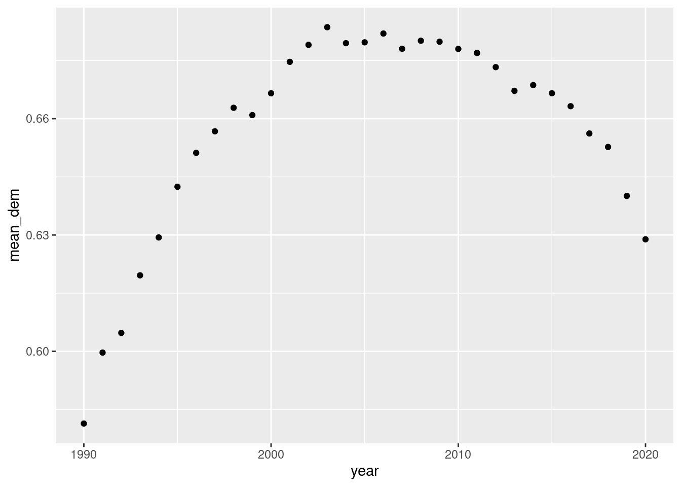
How can we visualize trends effectively? One alternative is to use a trend graph. Let’s start by computing the yearly averages for democracy in the whole region:
ggplot(dem_yearly, aes(x = year, y = mean_dem)) +geom_point()
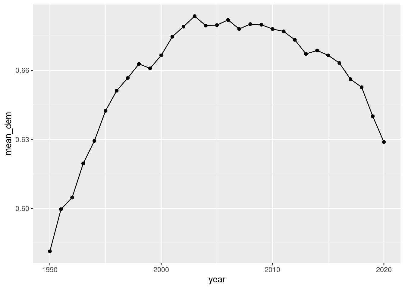
We can add geom_line() to connect the dots:
ggplot(dem_yearly, aes(x = year, y = mean_dem)) +geom_point() +geom_line()
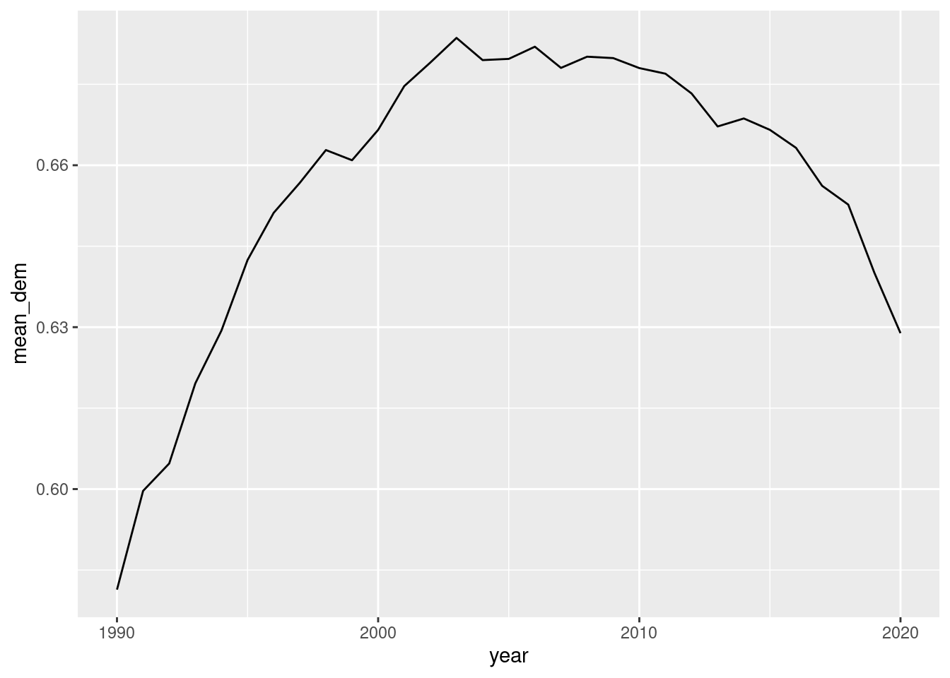
We can, of course, remove to points to only keep the line:
ggplot(dem_yearly, aes(x = year, y = mean_dem)) +geom_line()
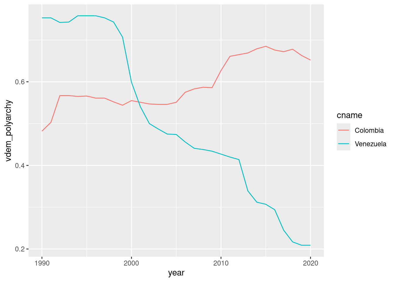
What if we want to plot trends for different countries? We can use the group and color aesthetic mappings (no need to do a summary here! data is already at the country-year level):
# filter to only get Colombia and Venezueladem_yearly_countries <- qog |>filter(ccodealp %in%c("COL", "VEN"))
ggplot(dem_yearly_countries, aes(x = year, y = vdem_polyarchy, color = cname)) +geom_line()
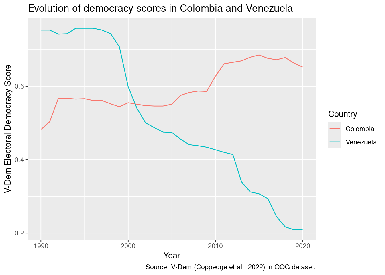
Remember that we can use the labs() function to add labels:
ggplot(dem_yearly_countries, aes(x = year, y = vdem_polyarchy, color = cname)) +geom_line() +labs(x ="Year", y ="V-Dem Electoral Democracy Score", color ="Country", title ="Evolution of democracy scores in Colombia and Venezuela",caption ="Source: V-Dem (Coppedge et al., 2022) in QOG dataset.")
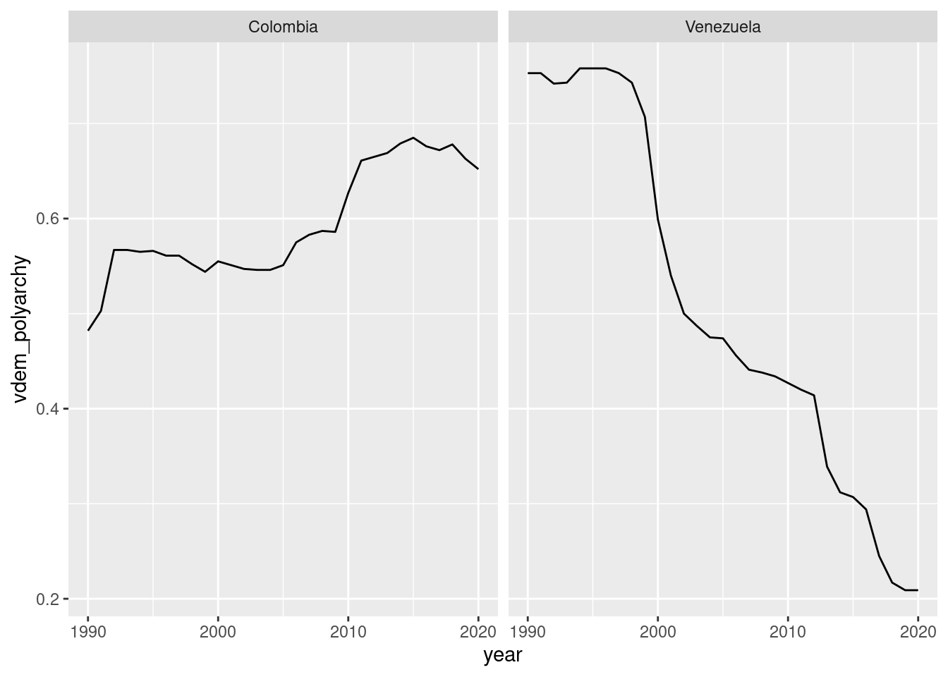
Another way to display these trends is by using facets, which divide a plot into small boxes according to a categorical variable (no need to add color here):
ggplot(dem_yearly_countries, aes(x = year, y = vdem_polyarchy)) +geom_line() +facet_wrap(~cname)
Facets are particularly useful for many categories (where the number of distinguishable colors reaches its limit):
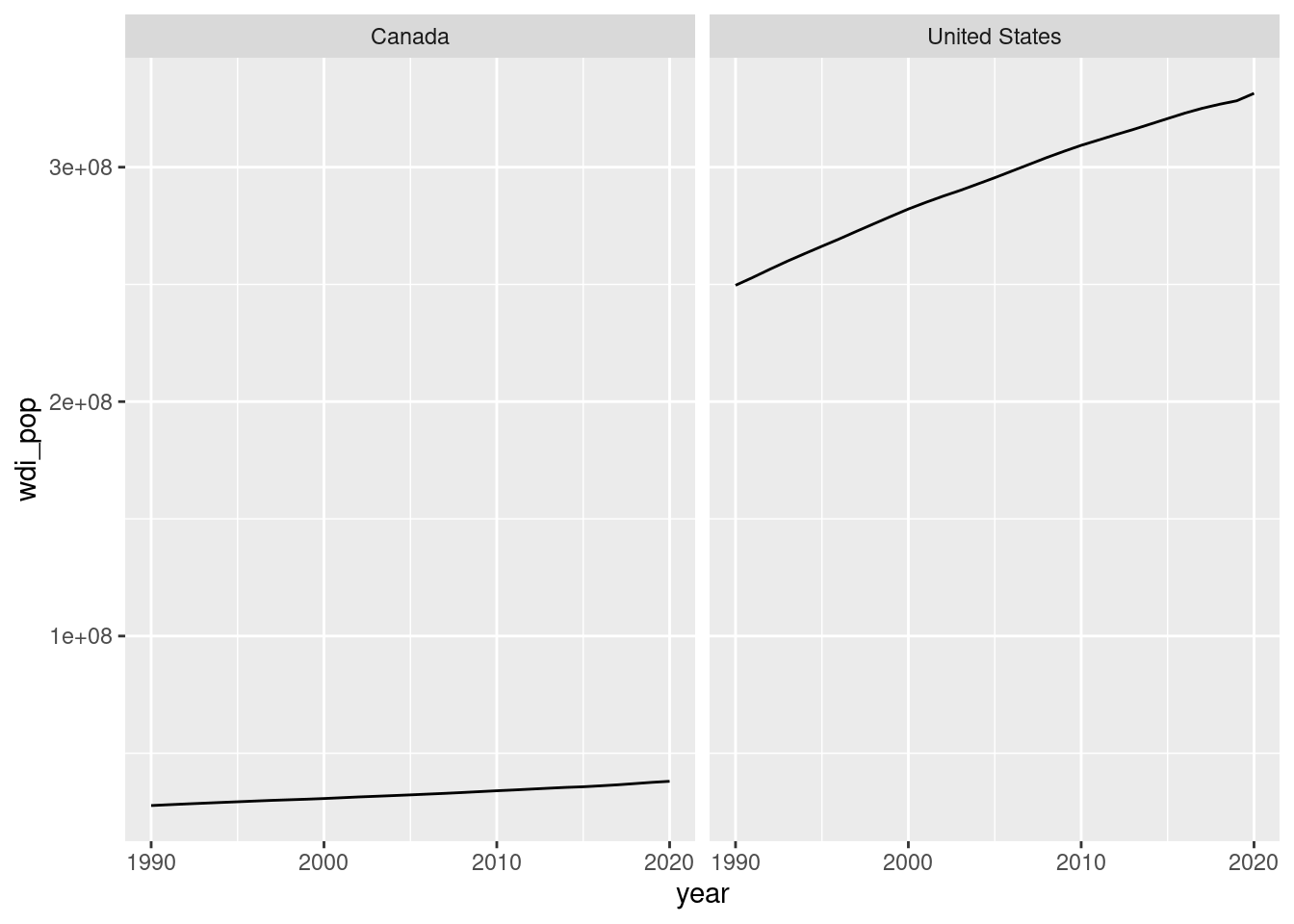
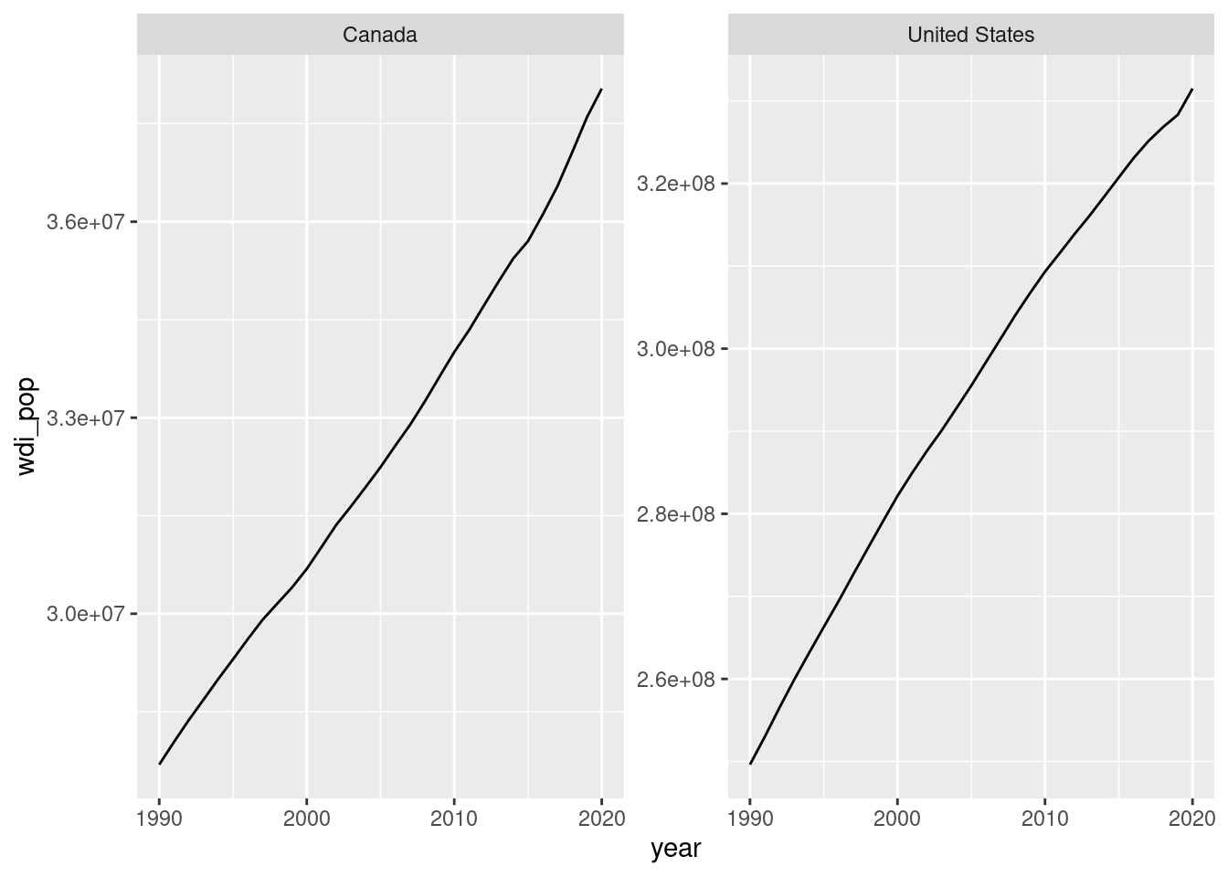
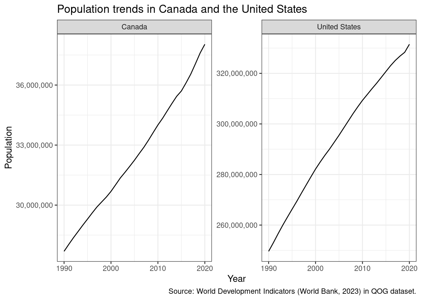
With facets, one can control whether each facet picks its own scales or if all facets share the same scale. For example, let’s plot the populations of Canada and the US:
The scales are so disparate that unifying them yields a plot that’s hard to interpret. But if we’re interested in within-country trends, we can let each facet have its own scale with the scales = argument (which can be “fixed”, “free_x”, “free_y”, or “free”):
This ability to visualize within time trends also makes facets appealing in many situations.
Tip
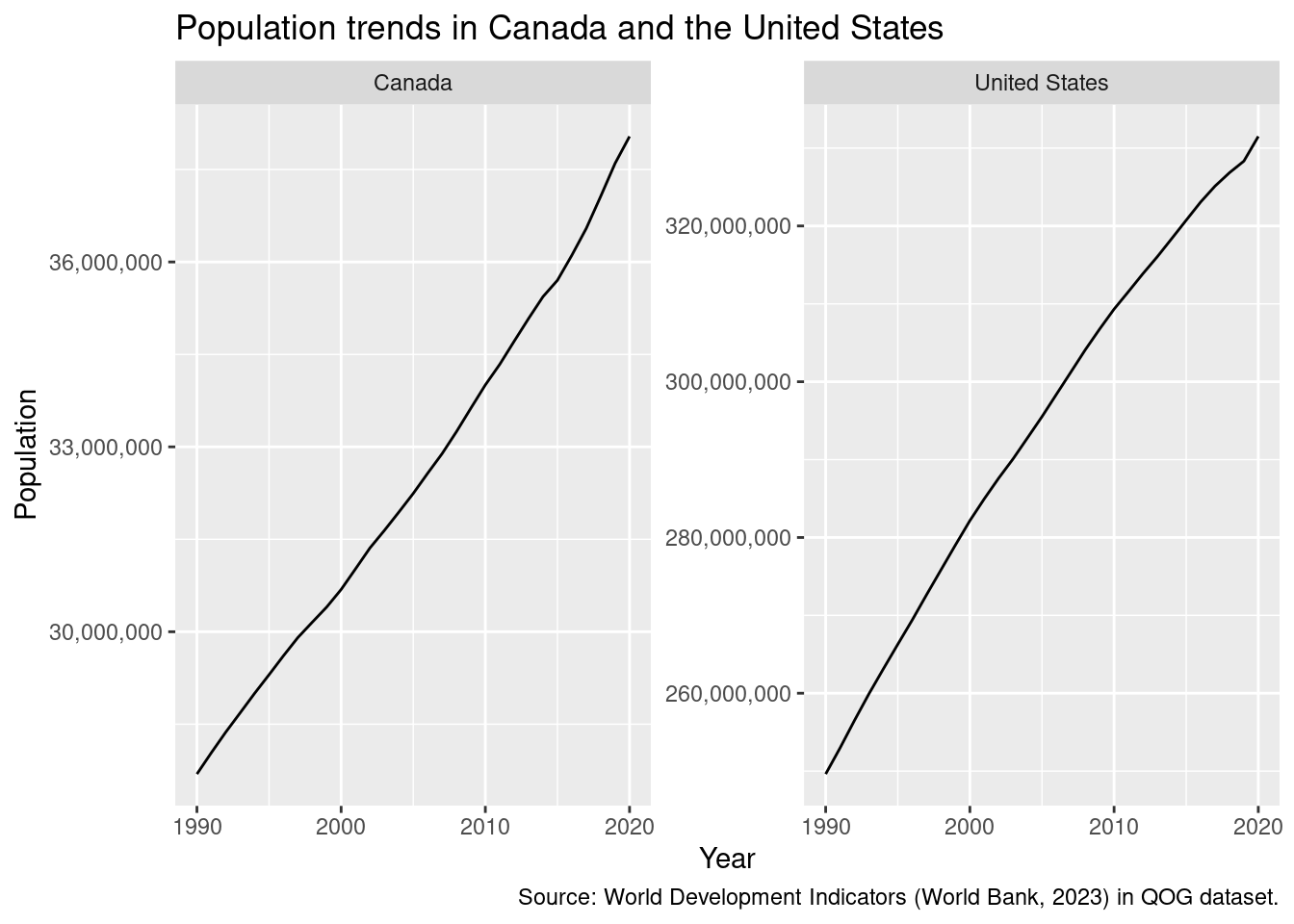
Plots made with ggplot2 are extremely customizable. For example, we could want to change the y-axis labels in the last plot to something more readable:
# create as object "p" to use laterp <-ggplot(qog |>filter(cname %in%c("Canada", "United States")), aes(x = year, y = wdi_pop)) +geom_line() +facet_wrap(~cname, scales ="free_y") +scale_y_continuous(labels = scales::label_number(big.mark =",")) +# also add labelslabs(x ="Year", y ="Population",title ="Population trends in Canada and the United States",caption ="Source: World Development Indicators (World Bank, 2023) in QOG dataset.")
While it’s impossible for us to review all the customization options you might need, a fantastic reference is the “ggplot2: Elegant Graphics for Data Analysis” book by Hadley Wickham, Danielle Navarro, and Thomas Lin Pedersen.
NoteExercise
Using your merged dataset from the previous section, plot the trajectories of C02 per capita emissions for the US and Haiti. Use adequate scales.
5.6.1 Themes
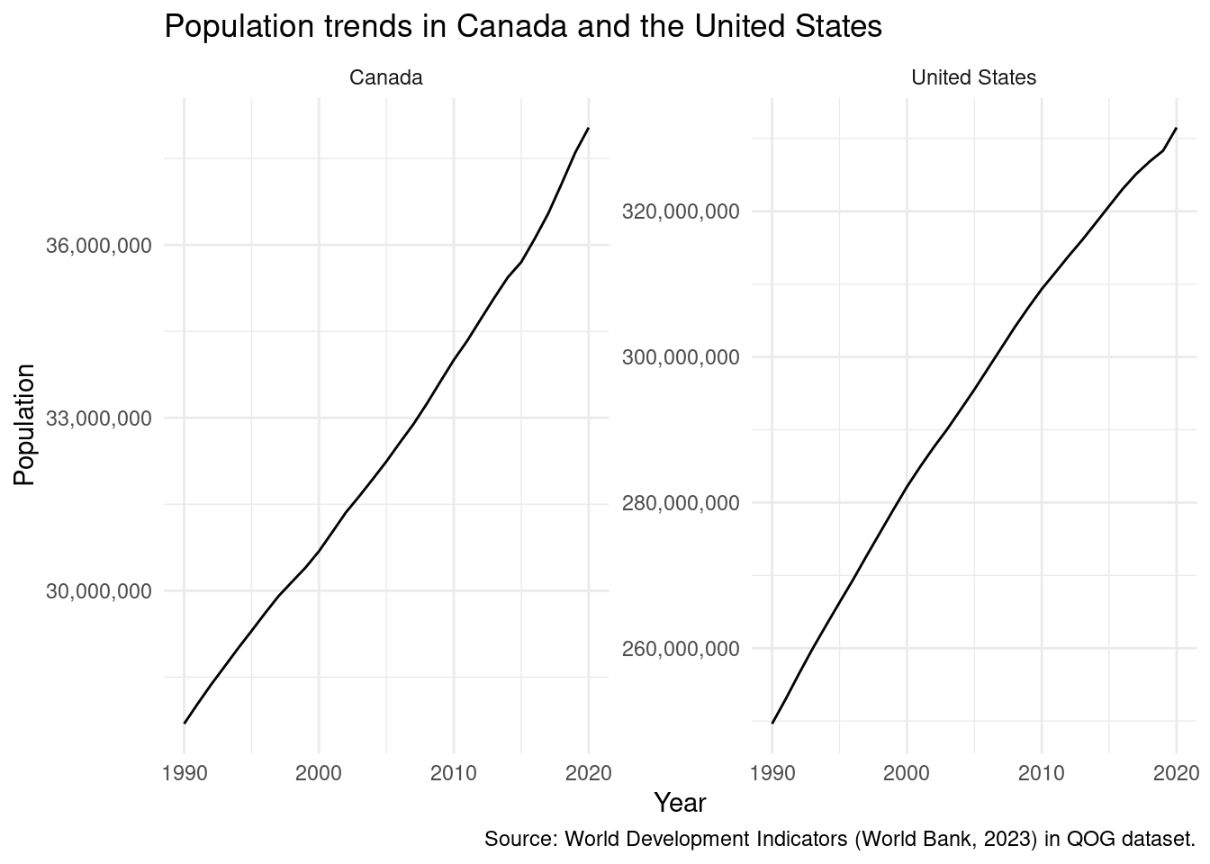
We can change the overall aspect of a ggplot2 figure by changing its theme:
p +theme_minimal()
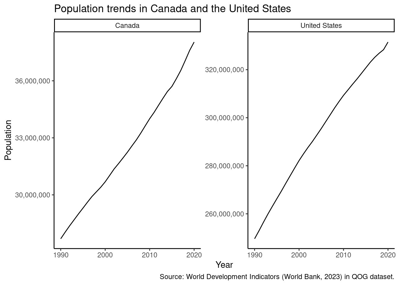
p +theme_classic()
p +theme_bw()
If you are going to make multiple plots in a script, you can set the theme at the beginning with theme_bw():
theme_set(theme_bw())p
Arel-Bundock, Vincent, Nils Enevoldsen, and CJ Yetman. 2018. “Countrycode: An r Package to Convert Country Names and Country Codes.”Journal of Open Source Software 3 (28): 848. https://doi.org/10.21105/joss.00848.
Aronow, Peter M, and Benjamin T Miller. 2019. Foundations of Agnostic Statistics. Cambridge University Press.
Baydin, Atılım Günes, Barak A. Pearlmutter, Alexey Andreyevich Radul, and Jeffrey Mark Siskind. 2017. “Automatic Differentiation in Machine Learning: A Survey.”The Journal of Machine Learning Research 18 (1): 5595–637.
Coppedge, Michael, John Gerring, Carl Henrik Knutsen, et al. 2022. V-Dem Codebook V12. Varieties of Democracy (V-Dem) Project. https://www.v-dem.net/dsarchive.html.
U. S. Department of Agriculture [USDA], Agricultural Research Service. 2019. Department of Agriculture Agricultural Research Service. https://fdc.nal.usda.gov/.
Whittinghill, Dexter C, and Robert V Hogg. 2001. “A Little Uniform Density with Big Instructional Potential.”Journal of Statistics Education 9 (2).
Wickham, Hadley, Danielle Navarro, and Thomas Lin Pedersen. 2023. Ggplot2: ElegantGraphics for DataAnalysis. 3rd ed. https://ggplot2-book.org/.
Technically, the read_csv() and read_rds() functions come from readr, one of the tidyverse constituent packages.↩︎
There are R packages to deal with these complications. fuzzyjoin matches units by their approximate distance, using some clever algorithms. countrycode allows one to standardize country names and country codes across different conventions.↩︎